Solution to Unit Commitment with Priority
List Approach
Manisha Govardhan
Research Scholar, Dept. of Electrical Engg, S.V. National Institute of Technology, Surat, Gujarat, India
ABSTRACT: Unit commitment problem (UCP) plays a key role in the power system operation and control. This paper deals with the mathematical formulation of conventional UCP and its solution with priority list (PL) approach using GABC algorithm. In this study, three different PL approaches are deliberated, namely, cost priority, power priority and hybrid priority to attain optimum solution. The optimal results ofUCP with different PL approaches are compared over a scheduling period which yields that the power priority and hybrid priority methods provide better result compared to the conventional cost priority approach for standard IEEE 10-unit system.
KEYWORDS:Cost priority (CP), Global best Artificial Bee Colony (GABC) algorithm, hybrid priority (HP), power priority (PP), unit commitment problem (UCP).
I. INTRODUCTION
Due to growing energy demand and limited generation resources, generation scheduling has become a challenging task for the utility and power system operators. In modern power system, unit commitment problem (UCP) is the most important and stimulating power system problem of daily generation planning. Due to the inconsistent nature of load demand, it becomes indispensable for the generation authorities to predict the generation scheduling in advance to obtain the economic and reliable system while satisfying the load demand. UCP combines two sub problems of power system such as unit commitment (UC) and economic load dispatch (ELD). UC decides when to start-up and shut down the generating units while ELD performs distribution of generated power among the committed units. Hence, the combine solution to UC and ELD as UCP is considered as the most challenging task due to its nonlinear and random nature that involves definite constraints, nonlinear objective function and enormous dimensions. Although, researchers extensively studied this complex problem from decades, the research is still ongoing on UCP and many methods and optimization techniques have been developed to solve the classic UCP. Exhaustive enumeration (EE) [1] selects the best solution by enumerating the all possible combinations of the generating units and hence, it is not suitable for large scale system and even for medium size UCP.
The traditional methods include priority list (PL) method [2-3], branch and bound (BB) method [4], dynamic programming (DP) [5], mixed-integer linear programming (MIP) [6] and Lagrangian Relaxation (LR) [7-8]. Among these traditional methods, the PL method is the simplest and fastest as it commits the generating units in ascending order of their average production cost. Hence, units with low generation cost are committed first. The BB method has a limitation of lack of storage capacity and computation time grows exponentially as the number of generating unit increases. The DP method is flexible and provides optimal solutions in small power systems. However, considering all constraints and possible combinations of generating units require enormous computation in large-scale power systems. The MIP method adopts linear programming techniques to obtain an integer solution which is imprecise to solve the non-linear UCP. The LR method attempts to obtain the appropriate co-ordination technique that generates feasible solution with reduced duality gap. Hence, the LR method suffers from convergence problem and poor quality solution due to the dual nature of the algorithm.
tothe GABC optimization algorithm is presented in section 3. Section 4 deliberates the simulation results and comparisons of different cases considered. Finally, the conclusion is drawn in section 5.
II. PROBLEM FORMULATION
The main objective of the classic UCP is to minimize the total cost of the system while satisfying the load demand, spinning reserve and other constraints over the scheduled time horizon as follows:
( , ) ( , ) ( ) ( , ) ( ) ( , )
1 1
min
(
)
G
N T
total i G i h i h i i h i i h h i
C
C P
U
SC x
SD y
(1)whereCtotaldescribes the total cost of the system. NG is specified as number of generating units and T is the schedule
time horizon. U(i,h) indicates the on/off status of ith unit at hour h and h signifies the hour index. x(i,h) and y(i,h) are the
start-up and shut down indicators of unit i at hour h respectively.
The operation cost of the system is an accumulation of the fuel cost, start-up cost and shut down cost of all committed units over the scheduled time period. The first term in equation (1) is the fuel cost of a generating unit which can be characterized in quadratic polynomial form as:
2 ( , ) ( , ) ( , )
(
)
i G i h i i G i h i G i h
C P
a
b P
c P
(2)where
a
i,
b
iandc
i are the fuel cost coefficients and PG(i,h) is the power output at hour h of ith generating unit. Thesecond and third terms describe the start-up and shut down costs of each generating unit respectively. Generally, shut down cost is constant for each unit and the start-up cost depends on boiler temperature of a thermal unit and can be specified as:
( ) ( , ) ( , ) ( , ) ( , ) ( )
( ) ( , ) ( , ) ( , ) off
i i h i h i h i h
i off
i i h i h i h
HSC
if
MD
U
MD
CSH
SC
CSC
if
U
MD
CSH
(3)
where U(i,h)off is the duration during which ith generating unit continuously remains off till hour h. HSC and CSC are
referred to as hot and cold start-up cost respectively. CSHi is cold start hour and MU(i,,h) and MD(i,,h) are minimum up
and down time of unit i at hour h respectively.The execution of the above UCP model must satisfy several constraints listed below:
A) Power balance constraint:The accumulation of power generated from all the committed units must satisfy the load demand at that particular interval and is characterized as:
( , ) ( , ) ( )
1
G
N
G i h i h L h i
P
U
P
(4)wherePL(h) is denoted as hourly load demand.
B) Generation limit constraint:For system stability and safe operation of each generating unit, the generated power must be within the specified lower and upper limits as follows:
min max
( ) ( ) ( ) G i G i G i
P
P
P
(5)wherePGminand PGmax are minimum and maximum generation capacities of each thermal unit respectively.
on i i
off
i i
U MU
U MD
(6)
whereUion and MU are the minimum on time and minimum up time respectively.
D) Spinning reserve constraint:Adequate spinning reserve (SR) should be required for stable and reliable operation. The SR constraint can be designed as:
max
( , ) ( , ) ( ) ( ) 1
G N
G i h i h L h h i
P
U
P
SR
(7)III. OVERVIEW OF GABC ALGORITHM
Karaboga has developed the basic concept of artificial bee colony algorithm which emphases the food finding habits of honeybees. The artificial bees are mainly distributed into three groups, namely, employed bees, onlookers and scouts [9]. These bees fly in multidimensional search space to pursue their food source. Employed bees use their own experience to find the food source while scout bees hunt their food source arbitrarily. The onlooker bees pick good food source from those founded by the employed bees and they further search food source nearby the selected food source. Each food source signifies the possible solution of the optimization problem and quality of the food source is judged by the nectar amount of the food source. In ABC,the initial population P of Np possible solution is generated randomly.
Each Pi (i= 1, 2,……Np) is a D dimensional vector where D is the number of optimized parameters. In employed bee
phase, the new random food source is generated as follows [10]:
( )
i j i j i j ij kj
v P P P (8)
wherePij andvij indicate the previous and new food source respectively andijdenotes a random number between 0 to
1, j € {1,2…D} and Pk indicates an alternative solution chosen randomly from the population. In GABC, global best
(gbest) solution is used to improve the search mechanism and the equation (22) is modified as [10]:
( ) ( )
i j i j i j ij kj ij j i j
v P P P y P (9)
The added term in (23) is gbest term, yj is the jth element of the global best solution and Ψij is a random number in [0,
C] where C is a nonnegative constant. In onlooker phase, each onlooker bee chooses a food source according to the probability value pi = fiti/ Σnfitn wherefit describes the fitness of a solution. Thereafter, onlooker bees further searches
for better solution (food source) in the neighborhood of the selected one according to (23). If the solution has not improved after certain trials, then scout bees generate new food source and repeat the hunting process.
IV. RESULT AND DISCUSSION
The conventional priority list (PL) method is considered to solve the UCP in this section. In this study, three different strategies of the priority selection of generating units are considered. The priority order of each generating unit is decided according to the cost priority (CP), power priority (PP) and hybrid priority (HP) [11].
Cost priority (CP): CP is the conventional priority list method based on Full load average production cost (FLAC) used
to solve the unit commitment problem. FLAC (α) is defined as the cost per unit of power when the unit is at its maximum capacity. α can be calculated as [1]:
max
max max max
(
)
i Gi i
i i i Gi
Gi Gi
f P
a
b
c P
P
P
The units are committed in ascending order of their αi. The thermal unit with lowest αi will have the highest priority to
commit. While decommitment of thermal units, reverse order is followed, i.e. the unit with the highest αi is withdrawn
first.
Power priority (PP): PP is based on the maximum power rating of the generating unit. The units are arranged according to their maximum generation capacities and unit with the highest power rating will have the first priority to commit and so on.
Hybrid priority (HP): In HP, hybrid strategy of CP and PP is applied. Initially, the priority of generating unit is decided according to the maximum power rating of the unit. Thermal unit with the highest power rating will have first priority. Then, this priority order is rearranged according to the traditional priority list method based on full load average cost (FLAC). Hence, the thermal units with higher generation limit and lowest FLAC will have the first priority.
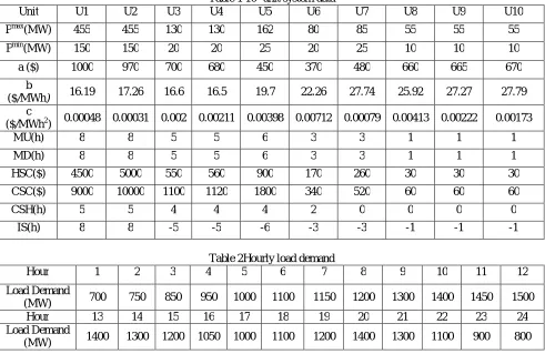
In this study, GABC is employed to solve the basic UCP using different priority approaches for standard IEEE 10 unit system. The generation characteristics of 10 unit system and 24 hours load demand data obtained from [12] are provided in Table 1 and Table 2 respectively. For system reliability, spinning reserve is assumed as 10% of the hourly load demand.
Table 1 10- unit system data
Unit U1 U2 U3 U4 U5 U6 U7 U8 U9 U10
Pmax(MW) 455 455 130 130 162 80 85 55 55 55
Pmin(MW) 150 150 20 20 25 20 25 10 10 10
a ($) 1000 970 700 680 450 370 480 660 665 670
b
($/MWh) 16.19 17.26 16.6 16.5 19.7 22.26 27.74 25.92 27.27 27.79
c
($/MWh2) 0.00048 0.00031 0.002 0.00211 0.00398 0.00712 0.00079 0.00413 0.00222 0.00173
MU(h) 8 8 5 5 6 3 3 1 1 1
MD(h) 8 8 5 5 6 3 3 1 1 1
HSC($) 4500 5000 550 560 900 170 260 30 30 30
CSC($) 9000 10000 1100 1120 1800 340 520 60 60 60
CSH(h) 5 5 4 4 4 2 0 0 0 0
IS(h) 8 8 -5 -5 -6 -3 -3 -1 -1 -1
Table 2Hourly load demand
Hour 1 2 3 4 5 6 7 8 9 10 11 12
Load Demand
(MW) 700 750 850 950 1000 1100 1150 1200 1300 1400 1450 1500 Hour 13 14 15 16 17 18 19 20 21 22 23 24 Load Demand
(MW) 1400 1300 1200 1050 1000 1100 1200 1400 1300 1100 900 800
Table 3 Priority order for 10 unit system
Units FLAC(αi) PGmax CP PP HP
U1 18.6062 455 1 1 1
U2 19.5329 455 2 2 2
U3 22.2446 130 4 5 5
U4 22.0051 130 3 3 4
U5 23.1225 162 5 4 3
U6 27.4546 80 6 7 7
U7 33.4542 85 7 6 6
U8 38.1472 55 8 8 8
U9 39.4830 55 9 9 9
U10 40.0670 55 10 10 10
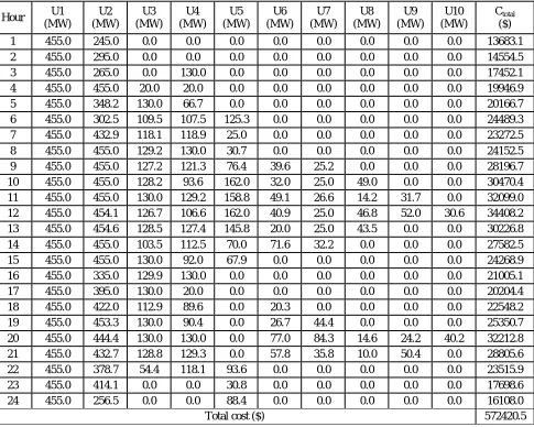
Table 4 Generation scheduling for CP
Hour U1 (MW)
U2 (MW)
U3 (MW)
U4 (MW)
U5 (MW)
U6 (MW)
U7 (MW)
U8 (MW)
U9 (MW)
U10 (MW)
Ctotal
($)
1 455.0 245.0 0.0 0.0 0.0 0.0 0.0 0.0 0.0 0.0 13683.1 2 455.0 295.0 0.0 0.0 0.0 0.0 0.0 0.0 0.0 0.0 14554.5 3 455.0 265.0 0.0 130.0 0.0 0.0 0.0 0.0 0.0 0.0 17452.1 4 455.0 455.0 20.0 20.0 0.0 0.0 0.0 0.0 0.0 0.0 19946.9 5 455.0 348.2 130.0 66.7 0.0 0.0 0.0 0.0 0.0 0.0 20166.7 6 455.0 302.5 109.5 107.5 125.3 0.0 0.0 0.0 0.0 0.0 24489.3 7 455.0 432.9 118.1 118.9 25.0 0.0 0.0 0.0 0.0 0.0 23272.5 8 455.0 455.0 129.2 130.0 30.7 0.0 0.0 0.0 0.0 0.0 24152.5 9 455.0 455.0 127.2 121.3 76.4 39.6 25.2 0.0 0.0 0.0 28196.7 10 455.0 455.0 128.2 93.6 162.0 32.0 25.0 49.0 0.0 0.0 30470.4 11 455.0 455.0 130.0 129.2 158.8 49.1 26.6 14.2 31.7 0.0 32099.0 12 455.0 454.1 126.7 106.6 162.0 40.9 25.0 46.8 52.0 30.6 34408.2 13 455.0 454.6 128.5 127.4 145.8 20.0 25.0 43.5 0.0 0.0 30226.8 14 455.0 455.0 103.5 112.5 70.0 71.6 32.2 0.0 0.0 0.0 27582.5 15 455.0 455.0 130.0 92.0 67.9 0.0 0.0 0.0 0.0 0.0 24268.9 16 455.0 335.0 129.9 130.0 0.0 0.0 0.0 0.0 0.0 0.0 21005.1 17 455.0 395.0 130.0 20.0 0.0 0.0 0.0 0.0 0.0 0.0 20204.4 18 455.0 422.0 112.9 89.6 0.0 20.3 0.0 0.0 0.0 0.0 22548.2 19 455.0 453.3 130.0 90.4 0.0 26.7 44.4 0.0 0.0 0.0 25350.7 20 455.0 444.4 130.0 130.0 0.0 77.0 84.3 14.6 24.2 40.2 32212.8 21 455.0 432.7 128.8 129.3 0.0 57.8 35.8 10.0 50.4 0.0 28805.6 22 455.0 378.7 54.4 118.1 93.6 0.0 0.0 0.0 0.0 0.0 23515.9 23 455.0 414.1 0.0 0.0 30.8 0.0 0.0 0.0 0.0 0.0 17698.6 24 455.0 256.5 0.0 0.0 88.4 0.0 0.0 0.0 0.0 0.0 16108.0
Table 5 Generation scheduling for PP Hour U1
(MW) U2 (MW) U3 (MW) U4 (MW) U5 (MW) U6 (MW) U7 (MW) U8 (MW) U9 (MW) U10 (MW) Ctotal ($) 1 455.0 245.0 0.0 0.0 0.0 0.0 0.0 0.0 0.0 0.0 13683.1 2 455.0 295.0 0.0 0.0 0.0 0.0 0.0 0.0 0.0 0.0 14554.5 3 455.0 370.0 0.0 0.0 25.0 0.0 0.0 0.0 0.0 0.0 17709.6 4 455.0 454.6 0.0 0.0 40.4 0.0 0.0 0.0 0.0 0.0 18598.6 5 455.0 388.2 130.0 0.0 26.7 0.0 0.0 0.0 0.0 0.0 20605.4 6 455.0 384.9 106.0 129.0 25.0 0.0 0.0 0.0 0.0 0.0 22397.6 7 455.0 409.8 130.0 130.0 25.2 0.0 0.0 0.0 0.0 0.0 24382.5 8 455.0 455.0 129.9 129.8 30.2 0.0 0.0 0.0 0.0 0.0 24150.9 9 455.0 445.3 130.0 129.0 95.6 20.0 25.0 0.0 0.0 0.0 28142.0 10 455.0 454.3 129.7 130.0 152.4 43.5 25.0 10.0 0.0 0.0 30140.6 11 455.0 454.7 126.6 129.4 162.0 77.3 25.0 10.0 10.0 0.0 32002.5 12 455.0 454.7 130.0 130.0 161.9 80.0 27.9 29.0 10.0 21.3 33975.7 13 455.0 455.0 129.8 128.5 162.0 27.5 25.0 17.1 0.0 0.0 30090.4 14 455.0 452.5 130.0 129.9 86.2 21.1 25.3 0.0 0.0 0.0 27263.5 15 455.0 455.0 130.0 130.0 30.0 0.0 0.0 0.0 0.0 0.0 24150.4 16 455.0 447.8 122.2 0.0 25.0 0.0 0.0 0.0 0.0 0.0 20930.4 17 455.0 407.8 112.2 0.0 25.0 0.0 0.0 0.0 0.0 0.0 20058.7 18 455.0 453.6 129.4 0.0 37.0 0.0 25.0 0.0 0.0 0.0 22828.6 19 455.0 451.4 128.5 0.0 118.6 20.0 26.5 0.0 0.0 0.0 25202.4 20 455.0 455.0 129.8 0.0 161.9 80.0 29.4 55.0 23.4 10.3 32021.3 21 455.0 454.9 128.1 130.0 86.9 20.0 25.0 0.0 0.0 0.0 27817.3 22 455.0 369.5 125.6 124.9 25.0 0.0 0.0 0.0 0.0 0.0 22390.9 23 455.0 315.0 0.0 130.0 0.0 0.0 0.0 0.0 0.0 0.0 17764.1 24 455.0 218.5 0.0 126.4 0.0 0.0 0.0 0.0 0.0 0.0 16022.9
Total cost ($) 566884.3
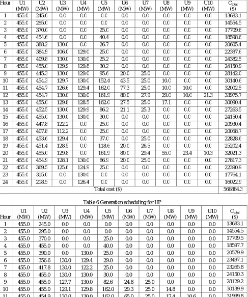
Table 6 Generation scheduling for HP
The comparison of total cost for different priority approaches employing GABC is given in Table 7 which shows that CP yields maximum cost whereas both PP and HP perform almost similar and result in lower cost compared to the CP.
Table 7 Comparison of total cost
Priority Total cost ($)
CP 572420.5
PP 566884.3
HP 566678.0
V.CONCLUSION
In this paper, three different priority list approaches, namely, cost priority (CP), power priority (PP) and hybrid priority (HP), are employed to solve the basic UCP with an effective GABC algorithm. In PL approach, it can be observed that the results obtained with PP and HP are almost similar and better than CP. The results confirm that PL method is simple, but may results in sub-optimal solution since it provides the schedule according to the predefined priority order as priority order of generating unitshas the great influence on the total cost. Also, PL method may leads to a solution with relatively higher generation cost because start-up cost and ramp rate limits are not considered in determining the priority order of the committed units. But, PL method proves simple and fast for large scale unit system.
REFERENCES
[1] A.J. Wood and B.F. Woolenberg, “Power generation, operation and control,” John Wiley and Sons, New York, N.Y., (1984).
[2] R. M. Burns and C. A. Gibson,“Optimization of priority lists for a unit commitment program,”IEEE Transactions on Power Apparatus and Systems, vol. 94, no.6, pp. 1917-1917, 1975.
[3] T. Senjyu, S. Kai, U. Katsumi and F. Toshihisa, “A fast technique for unit commitment problem by extended priority list,” IEEE Transactions on Power Systems, vol. 18, no. 2,pp. 882-888, 2003.
[4] A.I. Cohen and Y. Miki,“A branch-and-bound algorithm for unit commitment,” IEEE Transactions on Power Apparatus and Systems, vol.2,pp. 444-451, 1983.
[5] Z. Ouyangand S. M. Shahidehpour,“An intelligent dynamic programming for unit commitment application,” IEEE Transactions onPower Systems,vol. 6, no. 3, 1203-1209, 1991.
[6] H. Daneshi, L.C. Azim, M. Shahidehpourand Z. Li,“Mixed integer programming method to solve security constrained unit commitment with restricted operating zone limits,”IEEE International Conference on Electro/Information Technology (EIT), pp. 187-192, 2008.
[7] F. Zhuang and D. G. Frank, “Towards a more rigorous and practical unit commitment by Lagrangian relaxation,” IEEE Transactions on Power Systems, vol. 3, no. 2,pp.763-773, 1988.
12 455.0 455.0 130.0 130.0 162.0 79.9 26.9 37.1 10.0 14.1 33959.7 13 455.0 455.0 130.0 129.8 162.0 30.3 25.0 12.8 0.0 0.0 30067.8 14 455.0 451.5 124.6 127.8 96.0 20.0 25.0 0.0 0.0 0.0 27286.3 15 455.0 454.9 130.0 130.0 30.0 0.0 0.0 0.0 0.0 0.0 24150.4 16 455.0 437.1 0.0 130.0 27.9 0.0 0.0 0.0 0.0 0.0 20902.7 17 455.0 390.0 0.0 130.0 25.0 0.0 0.0 0.0 0.0 0.0 20020.0 18 455.0 453.6 0.0 130.0 36.1 0.0 25.2 0.0 0.0 0.0 22797.6 19 455.0 455.0 0.0 130.0 115.0 20.0 25.0 0.0 0.0 0.0 25144.2 20 455.0 455.0 0.0 130.0 162.0 80.0 26.6 54.9 25.9 10.5 31987.6 21 455.0 452.9 130.0 129.4 87.5 20.0 25.1 0.0 0.0 0.0 27809.5 22 455.0 383.9 109.2 126.9 25.0 0.0 0.0 0.0 0.0 0.0 22397.0 23 455.0 315.0 130.0 0.0 0.0 0.0 0.0 0.0 0.0 0.0 17795.3 24 455.0 215.0 130.0 0.0 0.0 0.0 0.0 0.0 0.0 0.0 16052.8
[8] S. Virmani, E.C. Adrian, KImhofand S. Mukherjee,“Implementation of a Lagrangian relaxation based unit commitment problem,” IEEE Transactions on Power Systems, vol. 4, no. 4, pp.1373-1380, 1989.
[9] B.Basturk and D. Karaboga, “An Artificial Bee Colony (ABC) Algorithm for Numeric function Optimization,”IEEE Swarm Intelligence Symposium, pp.12-14,2006.
[10] G. Zhu and S. Kwong, “Gbest-guided artificial bee colony algorithm for numerical function optimization,”Journal of Applied Mathematicsand Computation,vol. 217, pp. 3166-3173, 2010.
[11] A. Ahmad and A. Asar,“Unit Commitment Using Hybrid Approaches,” PhD diss., PhD Thesis, Department of Electrical Engineering, University of Engineering and Technology, Taxila, Pakistan, 2010.