Flows in Grooved Channels

(1)

Scholarship@Western

Electronic Thesis and Dissertation Repository

9-16-2013 12:00 AM

Flows in Grooved Channels

Alireza Mohammadi

The University of Western Ontario

Supervisor J. M. Floryan

The University of Western Ontario

Graduate Program in Mechanical and Materials Engineering

A thesis submitted in partial fulfillment of the requirements for the degree in Doctor of Philosophy

Follow this and additional works at: https://ir.lib.uwo.ca/etd

Part of the Mechanical Engineering Commons

Recommended Citation Recommended Citation

Mohammadi, Alireza, "Flows in Grooved Channels" (2013). Electronic Thesis and Dissertation Repository. 1626.

https://ir.lib.uwo.ca/etd/1626

This Dissertation/Thesis is brought to you for free and open access by Scholarship@Western. It has been accepted for inclusion in Electronic Thesis and Dissertation Repository by an authorized administrator of

(2)

(Thesis format: Monograph)

by

Alireza Mohammadi

Graduate Program in Mechanical and Materials Engineering

A thesis submitted in partial fulfillment of the requirements for the degree of

Doctor of Philosophy

The School of Graduate and Postdoctoral Studies The University of Western Ontario

London, Ontario, Canada

(3)

ii

Abstract

(4)

iii

the elimination of shear and results in an overall increase of drag. Potential for drag-reducing surfaces for this case exists if a method for reduction of undesired pressure and shear forces around groove tips can be found through proper shaping of the wall. Optimization method has been used in order to find forms of longitudinal grooves which minimize the flow losses in grooved channel and optimal shapes for different flow conditions have been identified.

Keywords

(5)

iv

Co-Authorship Statement

(6)

v

Dedication

(7)

vi

Acknowledgments

I greatly appreciate the unparalleled assistance and encouragement of my supervisor Prof. J. M. Floryan. Without his guidance and support the completion of this work would not have been possible.

I would like to express my gratitude to the members of my advisory committee, Prof. C. Zhang and Prof. E. Savory for their invaluable suggestions and constructive comments. I am also indebted to my colleagues Hadi Vafadar Moradi, Mohammad Fazel Bakhsheshi, Aidin Keikhaee, Syed Zahid Husain, David César Del Rey Fernandez, Ali Asgarian, German Kalugin and Mohammad Zakir Hossain for the insightful discussions that helped me during the achievement of this work. In particular, Hadi not only as my colleague but more importantly as my dearest friend has always supported me throughout the completion of my studies at the Western University.

(8)

vii

List of Figures

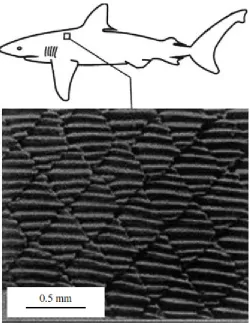
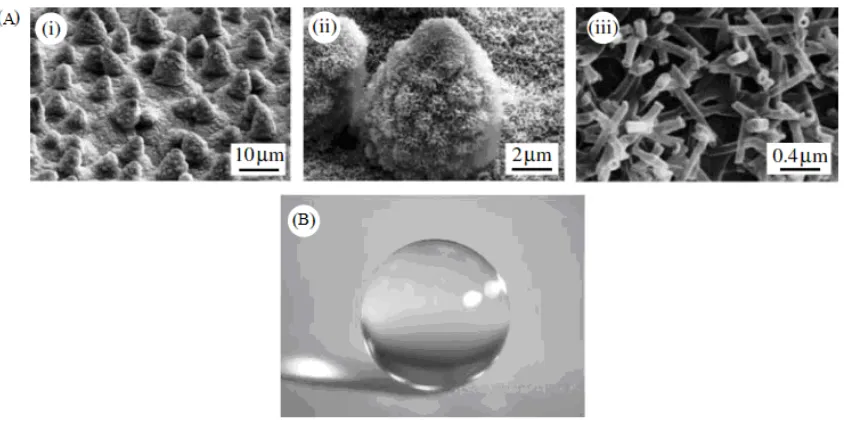
Figure 1.1: Tooth-like scale structure on a Galapagos shark (Bhushan 2009). ... 2 Figure 1.2: (A) Scanning electron microscope (SEM) micrographs (shown at three magnifications) of lotus leaf surface, which consists of microstructure formed by papillose epidermal cells covered with epicuticular wax tubules on the surface, which create nanostructure and (B) image of water droplet sitting on the lotus leaf (Bhushan 2009). ... 3

Figure 1.3: Hairs on the leaves of the water fern genus Salvinia are multicellular surface

structures. In (A) a water droplet on the upper leaf side of Salvinia biloba is shown. (B,C)

The crown-like morphology of the hairs of S. biloba (Bhushan 2009). ... 8

Figure 2.1: Channel with the grooved walls. The (xˆ,yˆ,zˆ) coordinate system is

flow-oriented and the (x,yˆ,z) system is groove-oriented. The angle

φ

shows the relative orientation of both systems. ... 21

Figure 2.2: Cross-section through the computational domain at z=const. It can be seen

that computational domain encloses the flow domain, where Yt and Yb denote the upper

and lower extremities of the flow domain. ... 31

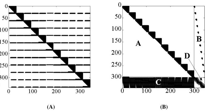
Figure 2.3: Structure of the coefficient matrix L for NM=5 and NT=30. The nonzero

elements are marked in black. The sparsity of L is 0.89. Figure 2.3A - the structure of the

coefficient matrix before the re-arrangement (see Eq. ( 2.74)), Figure 2.3B - the structure of the coefficient matrix after the re-arrangement (see Eq. ( 2.79a,b) and Section 2.4.1.3). ... 45

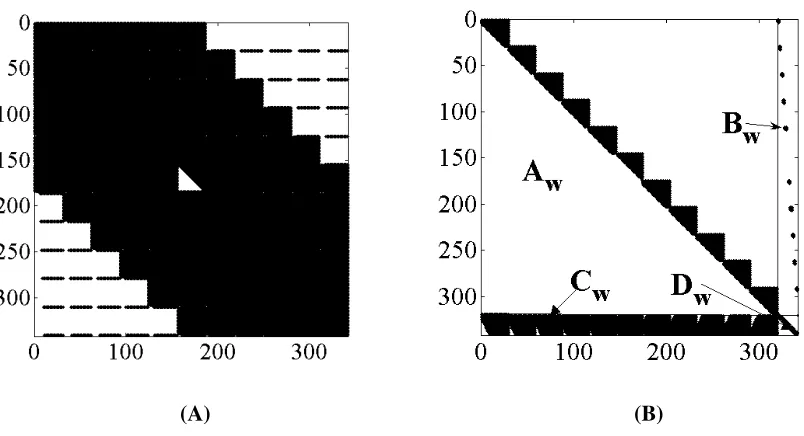
Figure 2.4: Structure of the coefficient matrices L1w (Figure 2.4A; see Eq. ( 2.81)) and

(13)

xii

Figure 2.5: Variations of the maximum error over the whole flow domain V _max (see Eq. ( 2.90)) as a function of the number of Chebyshev polynomials NT used in the computations for the model problem described by Eq. ( 2.89a,b) with the groove wavenumber

α

=2 and the groove orientation angle

φ

=30° for selected values of the groove amplitude S with the flow Reynolds number Re=50 (Figure 2.5A) and for selected

values of the flow Reynolds number Re with the groove amplitude S=0.01 and 0.025

(Figure 2.5B). All tests have been carried out using NM=20 Fourier modes. ... 51

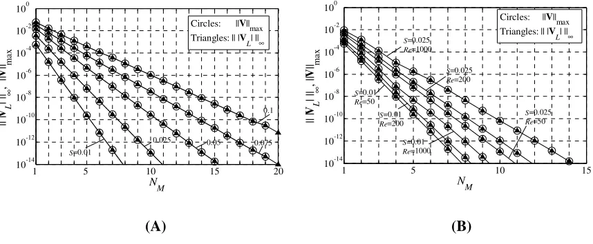
Figure 2.6: Variations of the maximum error over the whole flow domain V _max and the

maximum error at the grooved wall

∞

L

V as a function of the number of Fourier modes

NM used in the computations for the model problem described by Eq. ( 2.89a,b) with the

groove wavenumber

α

=2 and the groove orientation angle

φ

=30° for selected values of the groove amplitude S with the flow Reynolds number Re=50 (Figure 2.6A) and for

selected values of the flow Reynolds number Re with the groove amplitude S=0.01 and

0.025 (Figure 2.6B). All tests have been carried out using NT=70 Chebyshev polynomials.

It can be seen that

∞

= VL

V _max . ... 52

Figure 2.7: Distributions of the absolute value of the real part of the modal functions

DФ(n) (Figure 2.7A) and fw(n) (Figure 2.7B) for higher modes (n>15) in the region very close to the lower wall for the model geometry described by Eq. ( 2.89a,b) with the groove wavenumber

α

=5, the groove amplitude S=0.06, the flow Reynolds number

Re=50 and the groove orientation angle

φ

=30°. Formation of boundary layers around the grooved wall can be observed. Computations have been carried out using NM=20 Fourier modes and NT=70 Chebyshev polynomials. ... 53

Figure 2.8: Variations of the Chebyshev norms of the modal functions DФ(n) (Figure

2.8A) and fw(n) (Figure 2.8B) as a function of the Fourier mode number for the model geometry described by Eq. ( 2.89a,b) with the groove wavenumber

α

=1, the flow

Reynolds number Re=50 and selected values of the groove amplitudes S. Computations

(14)

xiii

Figure 2.9: Distributions of velocity components computed at the grooved wall uL(x), vL(x) and wL(x) for the model geometry described by Eq. ( 2.89a,b) with the groove

wavenumber

α

=5, the groove amplitude S=0.06 and the groove orientation angle

φ

=30°. Computations have been carried out using NM=20 Fourier modes and NT=70 Chebyshev polynomials... 54

Figure 2.10: Fourier spectra of velocity components computed at the grooved wall uL(x),

vL(x) and wL(x) for the model geometry described by Eq. ( 2.89a,b) with the groove wavenumber

α

=5, the groove amplitude S=0.06 and the groove orientation angle

φ

=30°. Computations have been carried out using NM=20 Fourier modes and NT=70 Chebyshev polynomials... 55

Figure 2.11: Fourier spectra of the streamwise uL(x) (Figure 2.11A) and the spanwise wL(x) (Figure 2.11B) velocity components for the model geometry described by Eq.

( 2.89a,b) with the groove amplitude S=0.05 and the groove wavelength λx=2π/3.

Solutions have been obtained in case A using computational box of length 2π/3 and NM=10 Fourier modes, in case B using computational box of length 4π/3 and NM=20

Fourier modes, and in case C using computational box of length 6π/3 and NM=30 Fourier

modes (see text for details). The presented results are for the flow Reynolds number

Re=50 and the groove orientation angle

φ

=30°. Computations have been carried out using

NT=70 Chebyshev polynomials... 56

Figure 2.12: Variations of the maximum boundary error

∞

L

V as a function of the groove wavenumber

α

for selected values of the groove amplitude S (Figure 2.12A) and

as a function of groove amplitude S for selected values of the groove wavenumber

α

(Figure 2.12B) for the model problem described by Eq. ( 2.89a,b). Dashed and solid lines correspond to results obtained with NM=15 and NM=20 Fourier modes, respectively. All

computations have been carried out using NT=70 for the flow Reynolds number Re=50

and the groove orientation angle

φ

=30°... 57

∞

L

(15)

xiv

as a function of the groove amplitude S for selected values of the groove wavenumber

α

(Figure 2.13B) for the model configuration described by Eq. ( 2.89a,b). All computations have been carried out using NM=20 Fourier modes and NT=70 Chebyshev polynomials for the flow Reynolds number Re=50. ... 58

∞

L

V as a function of the flow

Reynolds number Re for the model configuration described by Eq. ( 2.89a,b) with the

groove wavenumber

α

=4 and the amplitude S=0.04. Computations have been carried out

using the number of Fourier modes NM shown in figure and NT=70 Chebyshev

polynomials. The error does not depend on Re for

φ

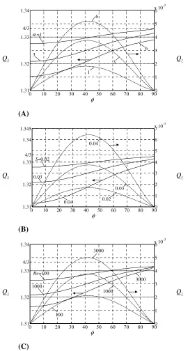
=90° (longitudinal grooves)... 59

Figure 2.15: Variations of the volume flow rate per unit width Qxˆ in the reference flow direction (xˆ -direction, solid lines) and of the volume flow rate Q_z_ˆ in the orthogonal

direction (zˆ -direction, dashed lines) as a function of the groove inclination angle

φ

. Figure 2.15A – Re=1000, S=0.03 and typical values of the groove wavenumber

α

. Figure 2.15B – Re=1000,

α

=3 and typical values of the groove amplitude S. Figure 2.15C –

α

=3, S=0.03 and typical values of the flow Reynolds number Re. All computations have

been carried out using NM=20 Fourier modes and NT=70 Chebyshev polynomials. ... 60

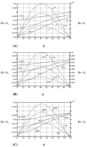
Figure 2.16: Variations of the pressure correction factors Re∗h_x_ˆ (solid lines) and

z

h

Re∗ _ˆ (dashed lines) as functions of the groove inclination angle

φ

. Figure 2.16A –

Re=1000, S=0.03 and typical values of the groove wavenumber

α

. Figure 2.16B – Re=1000,

α

=3 and typical values of the groove amplitude S. Figure 2.16C –

α

=3, S=0.03

and typical values of the flow Reynolds number Re. All computations have been carried

out using NM=20 Fourier modes and NT=70 Chebyshev polynomials... 62

Figure 3.1: Sketch of the flow system. ... 65

Figure 3.2: Variations of the norm v _max(see Eq. ( 3.16)) as a function of the corrugation

(16)

xv

Figure 3.3: Distributions of the x- and y-velocity components, i.e, u/c and v/(

α

*c), as a function of

η

at

ξ

= π/2 for the corrugation amplitude A = 0.2 for the flow Reynolds

numbers Re = 0.1 and Re = 1000 for the fixed flow rate constraint (Q1=0). In the above

1 ] 2 ) cos( 1

[ −

−

=M A ξ /

c . Solid and dashed lines identify numerical and asymptotic solutions, respectively... 70

Figure 3.4: Distributions of the x-component of surface stresses at the lower wall for the

corrugation amplitude A = 0.2 for the flow Reynolds numbers Re = 0.1 and Re = 1000

for the fixed flow rate constraint (Q1=0). Solid and dashed lines identify numerical and

asymptotic solutions, respectively. ... 72

Figure 3.5: Distributions of the y-component of pressure (

α

* Re)*dFy,pres at the lower wall for corrugations with the amplitude A = 0.2 for the flow Reynolds numbers Re = 0.1

and 1000 for the fixed flow rate constraint (Q1 = 0). Solid and dashed lines identify

numerical and asymptotic solutions, respectively. ... 73

Figure 3.6: Variations of the total force per unit channel length (Re/

λ

)*Ftotal and its various components (see Eqs ( 3.28)–( 3.31)) as a function of the corrugation amplitude A. Curves 1, 2, 3, 4, 5 and 6 correspond to (Re/

λ

)*Ftotal, (Re/

λ

)*Fs, (Re/

λ

)*Fform, (Re/

λ

)*Finter, (Re/

λ

)*Ftotal,1 and (Re/

λ

)*Fs,1. Dashed lines illustrate results of small-A

linearization of the total and form drags. Solid lines correspond to corrugation placed on one wall only. Dashed-dotted lines illustrate situation with corrugations placed on both walls (see Section 3.5). ... 76

Figure 3.7: Variations of fractions of contributions of the form, interaction and friction drags (see Eq. ( 3.32)) to the total drag as functions of the corrugation amplitude A. Solid

and dashed-dotted lines correspond to the corrugation placed on one wall only and placed on both walls, respectively... 76

Figure 3.8: Variations of the total force per unit channel length (Re/

λ

)*Ftotal and its

(17)

xvi

corrugation amplitudes A=B=0.5. Curves 1, 2, 3, 4, 5 and 6 correspond to (Re/

λ

)*Ftotal, (Re/

λ

)*Fs, (Re/

λ

)*Fform, (Re/

λ

)*Finter, (Re/

λ

)*Ftotal,1 and (Re/

λ

)*Fs,1, respectively. ... 82

Figure 4.1: A channel with grooved walls. Here (x,y,z) and (x~,y,~z) are the

flow-oriented and the groove-flow-oriented systems. The inclination angle

φ

shows the relative orientation of the two systems. ... 86

Figure 4.2: Sketch of the test configuration. The lower wall is fitted with sinusoidal

transverse grooves (

φ

= 0°; see Eq. ( 4.26)) kept at the average positions Save= 0.03, 0, −0.03 in cases A, B and C, respectively. ... 93

Figure 4.3: Variations of f1x*Re as a function of S for

α

= 0.1, 1, 5 for Re=0.01 (Figure

4.3A) and Re=1000 (Figure 4.3B). Other conditions are as in Figure 4.2. ... 94

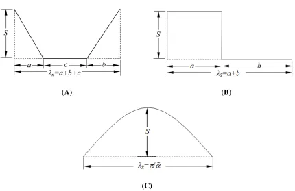
Figure 4.4: Sketch of the grooves used in the analysis. Triangular/trapezoidal, rectangular and rectified (described by |sin(α~~x)|) shapes are shown in Figure 4.4A, Figure 4.4B and Figure 4.4C, respectively. ... 95

Figure 4.5: Variations of f1x*Re (solid lines) and f1z*Re (dashed lines) as functions of the number of Fourier modes NA used to describe the groove geometry for Re=0.01 (Figure

4.5A) and Re=1000 (Figure 4.5B)for grooves with S = 0.02, α~=1, φ = 45° and shapes shown in Figure 4.4. Groove A: triangular shape (Figure 4.4A with a=b=π, c=0). Groove

B: trapezoidal shape (Figure 4.4A with a=b=c=2π/3). Groove C: rectangular shape (Figure 4.4B with a=b=π). Groove D: rectified shape (Figure 4.4C)... 96

Figure 4.6: Variations of f1x*Re (solid lines) and f1z*Re (dashed lines) as functions of φ for a channel with the grooves defined by Eq. ( 4.28). Figure 4.6A– Re = 1000, S = 0.06;

Figure 4.6B – Re = 1000, α~=3; Figure 4.6C –α~=3, S = 0.06... 99

Figure 4.7: Variations of f1x*Re (solid lines) and f1z*Re (dotted lines) as functions of φ

and α~ (Figure 4.7A) for the groove geometry defined by Eq. ( 4.28) with S=0.05 and

Re=500, as functions of φ and S for α~=3 and Re=500 (Figure 4.7B), and as functions of

(18)

xvii

Figure 4.8: Variations of f1x*Re (Figure 4.8A) and f1z*Re (Figure 4.8B) as functions of

α~ and S for a channel with shape defined by Eq. ( 4.28) for Re =500. Solid, dashed and dashed-dotted lines correspond to grooves with φ = 30°, 45°, 60°, respectively. ... 101

Figure 4.9: Distributions of the local shear force Re*tx,visc (Figure 4.9A) and the local

pressure force Re*tx,pres (Figure 4.9B) acting at the lower wall and the local shear force Re*gx,visc acting at the upper wall (Figure 4.9C) for transverse grooves with the shape

defined by Eq. ( 4.29) with S=0.05. Solid and dashed-dotted lines correspond to Re=0.01

and Re=1000, respectively. Dashed and dotted lines identify asymptotic (α→0) and smooth wall values, respectively. ... 105

Figure 4.10: Variations of the drag force per unit channel length (Re/λ)*Ftotal and its various components as a function of α for transverse grooves with S=0.05 (Figure 4.10A

– small α, Figure 4.10B – large α). Curves 1, 2, 3, 4, 5 and 6 correspond to (Re/λ)*Ftotal,

(Re/λ)*Fs, (Re/λ)*Fform, (Re/λ)*Finter, (Re/λ)*Ftotal,1 and (Re/λ)*Fs,1, respectively (see text

for explanations). Solid and dashed lines correspond to Re=0.01 and Re=1000, respectively. ... 107

Figure 4.11: Variations of fractions of the total drag created by different physical mechanisms (see Eq. ( 4.43)) as a function of α (Figure 4.11A - small α, Figure 4.11B - large α). Other conditions are as in Figure 4.10. ... 108

Figure 4.12: Distributions of the shear force Re*tx,visc (Figure 4.12A) and the pressure

force Re*tx,pres (Figure 4.12B) acting at the lower wall for transverse grooves with large

α. Circles identify flow separation and re-attachment points. Other conditions are as in Figure 4.9. Figure 4.12C displays variations of the shear force acting at the upper wall at two locations, i.e. above the trough and above the tip of the groove, as a function of α. ... 109

Figure 4.13: Streamlines (solid lines) and lines of constant pressure Re*p (dashed lines)

(19)

xviii

grooves with α=50 (Figure 4.13A) and α=100 (Figure 4.13B). Circles identify flow separation and re-attachment points... 110

Figure 4.14: Variations of f1x*Re as a function of αfor transverse grooves with the shape

defined by Eq. ( 4.29). The limit points for α→0 are 7.5×10−5, 3×10−4 and 1.876×10−3 for

S = 0.01, 0.02 and 0.05, respectively. The limit points represented by a channel with the lower wall shifted upwards by S/2 are 3.015×10−2, 6.061×10−2 and 1.538×10−1 for S = 0.01, 0.02 and 0.05, respectively. Solid and dashed lines correspond to Re=0.01 and Re=1000. ... 112

Figure 4.15: Variation of the equivalent channel opening ECh (see text for definition) as a

function of α. Other conditions are as in Figure 4.14. Limit points are represented by ECh

= 2 − S/2. ... 112

Figure 4.16: Variations of f1x*Re as a function of S for transverse grooves with α = 100 (solid lines) and α = 50 (dashed lines). Results for Re = 0.01, 1000 are displayed but they

overlap within the resolution of the figure. Contributions of different drag formation mechanisms are shown only for α = 100. Dashed lines represent reference curves proportional to S and S2. Figure 4.16A – the average position of the grooves is at y = −1.

Contributions of the shear drag and the pressure form drag are negative and are multiplied by −1 for convenience of the presentation. Figure 4.16B – tips of the grooves are located at y = −1. Contribution of the pressure interaction drag is positive and is multiplied by −1 for presentation purposes. The dashed-dotted line identifies the friction factor corresponding to a smooth channel with the lower wall located at yL=−1−S/2.... 114

Figure 4.17: Shapes used in the analysis of the effects of tilting of the transverse grooves. Configurations 1, ..., 11 correspond to b/λ = 0, 1/8, 1/4, 1/3, 5/12, 1/2, 7/12, 2/3,

3/4, 7/8, 1, respectively. Distribution of these grooves is illustrated in Figure 4.4A with

c=0. ... 115

Figure 4.18: Variation of the modification friction factor f1x*Re as a function of tilting of

(20)

xix

the lower wall with α=3 and S=0.05. The average position of the lower wall is kept the same and equal to y=−1 in all cases. ... 116

Figure 4.19: Variations of the friction factor f1x*Re in a channel with transverse triangular grooves with various tilting (see Figure 4.4A, c=0, and Figure 4.18) placed at the lower wall as a function of the grooves' wavenumber α and grooves' amplitude S for

the flow Reynolds number Re=500 (Figure 4.19A) and as a function of the flow Reynolds number Re and the amplitude S (Figure 4.19B) for the grooves' wavenumber α=3. Data

corresponding to configurations 1, 6 and 11 from Figure 4.17 is marked using dashed, solid and dashed-dotted lines, respectively. The average position of the lower wall is kept the same and equal to y = −1 in all cases. ... 116

Figure 4.20: Variations of the modification friction factor f1x*Re as a function of the

distance nc between individual grooves. Channel has flat upper wall and transverse

triangular grooves with shape shown in Figure 4.4A with S = 0.05, a = b = π/3, nc =

c/(a+b) either "glued" to the lower wall (solid lines) or "cut into" this wall (dashed-dotted

lines). Figure 4.20A - bases of the grooves are always kept at y = −1. Figure 4.20B - the

average channel opening is kept constant and equal to 2. Dotted lines in Figure 4.20A denote the effect of change in the average channel opening on f1x*Re... 118

Figure 4.21: Distribution of the local shear force Re*tx,tot acting at the lower (Figure

4.21A) and upper (Figure 4.21B) walls for longitudinal grooves with geometry defined by Eq. ( 4.44) with S=0.05 (solid lines). Dashed and dotted lines identify asymptotic

(β→0) and smooth wall (S=0) values, respectively... 120

Figure 4.22: Distribution of the u-velocity in a channel with longitudinal grooves defined by Eq.( 4.44) with S=0.05. Dotted, dashed-dotted and solid lines correspond to grooves with β → 0, 0.96, 5, respectively. Figure 4.22B provides enlargement of the middle section of Figure 4.22A... 121

Figure 4.23: Variations of f1x*Re induced by the longitudinal grooves with the shape

(21)

xx

Figure 4.23B– solid line: f1x*Re as a function of β for S=0.05, dashed lines: f1x*Re as a

function of S for β = 0.1, 3. The asymptote for β→0 is f1x*Re=−9.3728×10−4. ... 122

Figure 4.24: Variations of the modification friction factor f1x*Re as a function of the inclination angle φ for grooves with the shape defined by Eq. ( 4.28) with S=0.05 and the

small wavenumbers α~... 123

Figure 4.25: Variations of the modification friction factor f1x*Re as a function of the

grooves' amplitude S and wavenumber β for a channel with longitudinal grooves of triangular form placed at the lower wall. Shape of the grooves is given in Figure 4.4B with c = 0 and the average position of the lower wall is kept at y=−1. Figures 4.25A,

4.25B, 4.25C and 4.25D give results for configurations 6, 9, 10 and 11 from Figure 4.17, respectively. Drag reduction occurs for β <~ 0.92, 0.82, 0.67, 0.47 in each of these cases, respectively, regardless of the amplitude of the grooves... 124

Figure 4.26: Distribution of the local shear force Re*tx,tot acting at the lower wall for longitudinal grooves with medium β (Figure 4.26A) and large β (Figure 4.26B). Other conditions are as in Figure 4.21. Figure 4.26C displays variations of the local shear force

Re*gx,tot acting at the upper wall at two locations, i.e. above the trough and above the tip

of the groove, as a function of β. ... 125

Figure 4.27: Distribution of the u-velocity in a channel with longitudinal grooves.

Dotted, dashed-dotted and solid lines correspond to grooves with β = 10, 100, 200, respectively. Other conditions are as in Figure 4.22. Figure 4.27B provides enlargement of the bottom section of Figure 4.27A. ... 126

Figure 4.28: Channel with longitudinal grooves with shape defined by Eq. ( 4.44). Left

axis: variations of f1x*Re as a function of β. The limit points for β→0 are −3.75×10−5,

−1.5×10−4 and −9.373×10−4 for S = 0.01, 0.02 and 0.05, respectively. The limits for β→∞

are represented by smooth channel with the lower wall shifted upwards by S/2; they are 3.015×10−2, 6.061×10−2 and 1.538×10−1 for S = 0.01, 0.02 and 0.05, respectively. Right

(22)

xxi

function of β. Limit points for β→∞ are represented by ECh = 2 − S/2, i.e. they correspond to a smooth channel with the lower wall shifted upwards by distance S/2. . 127

Figure 4.29: Variations of f1x*Re as a function of S for longitudinal grooves. Dashed lines provide reference curves proportional to S and S2. Figure 4.29A – the average groove location is y = −1. Figure 4.29B – tips of the grooves are located at y = −1. The dashed-dotted line describes the friction factor for a smooth channel with the lower wall located at yL=−1−S/2. ... 128

Figure 4.30: Variations of the modification friction factor f1x*Re as a function of the

distance nc between individual grooves. Channel has flat upper wall and longitudinal triangular grooves with shape shown in Figure 4.4A with S = 0.05, a = b = π/3, nc =

c/(a+b) either "glued" to the lower wall (solid lines) or "cut into" this wall (dashed-dotted

lines). Figure 4.30A - bases of the grooves are always kept at y = −1. Figure 4.30B - the

average channel opening is kept constant and equal to 2. Dotted line in Figure 4.30A denotes the effect of change in the average channel opening on f1x*Re. ... 129

Figure 5.1:. Sketch of the flow configuration... 133 Figure 5.2: Variations of the errors ||u||_max (Figure 5.2A) and f₁_,_err (Figure 5.2B) of the

asymptotic solutions defined by Eq. ( 5.33a,b) for a channel with groove geometry described by Eq.( F.1a,b) for several values of A with B=A/2, φA=π/5, φB=π/3 as a function of the groove wavenumber β. ... 142

Figure 5.3: Variations of the normalized modification friction factor f1/f0 induced by the

(23)

xxii

Figure 5.4: Variation of the normalized modification friction factor f1/f0 for equal-depth

grooves located on the lower wall with S = 1 as a function of the number of Fourier

modes NA used in the description of the groove geometries... 147

Figure 5.5: Evolution of the optimal shape of the equal-depth grooves as a function of

the groove depth for the groove wavenumbers β close to transition between the drag reducing and drag increasing grooves. Results for β = 0.1, 0.5, 0.6, 0.7, 0.8, 0.9 are displayed in Figures 5.5A, 5.5B, 5.5C, 5.5D, 5.5E, and 5.5F, respectively. The y -coordinate is scaled using the peak-to-bottom distance as the length scale

) 2 ( ) 1

(y S / S

y_L = _L+ − . Thick lines illustrate the best-fitted trapezoids. These trapezoids are characterized by a=b=λ/11 and c=d=4.5λ/11, a=b=λ/8 and c=d=3λ/8, a=b=λ/7 and c=d=2.5λ/7, a=b=λ/6 and c=d=2λ/6, a=b=λ/5 and c=d=1.5λ/5, and a=b=λ/4 and c=d=λ/4

for β = 0.1, 0.5, 0.6, 0.7, 0.8 and 0.9, respectively. ... 150

Figure 5.6: Variations of the normalized modification friction factor f1/f0 as a function of

the groove wavenumber β and the groove depth S for a channel with the lower wall fitted

with the equal-depth grooves approximated by a trapezoid with a = b = λ/8 and c = d =

3λ/8 (solid lines). Results for the simple sinusoidal grooves are illustrated using dashed lines. Dotted lines identify values for β → 0 for the trapezoidal grooves (see Section 5.3.2). ... 151

Figure 5.7: Variations of the normalized modification friction factor f1/f0 as a function of

the groove wavenumber β for the equal-depth grooves located on the lower wall. Solid and dashed lines correspond to grooves with the optimal and trapezoidal shapes, respectively. ... 152

Figure 5.8: Contour plots of the velocity fields (Figure 5.8A) for the equal-depth optimal grooves (solid lines) and for the sinusoidal grooves (dashed lines) with S = 1, β = 0.5.

(24)

xxiii

for the optimal groove, the sinusoidal groove and the reference smooth wall, respectively. Lines a and b identify locations of the change in the wall curvature sign and the wall bottom “corner” for the optimal groove, respectively. ... 153

Figure 5.9: Shapes of the optimal grooves for a channel with both walls fitted with the

equal-depth grooves subject to constraints ( 5.39) with S = 0.4, 0.8 for β = 0.1 (Figure

5.9A) and β = 0.5 (Figure 5.9B). Thick lines illustrate the best-fitted trapezoid with a = b

= λ/8 and c = d = 3λ/8. The vertical coordinates are scaled with the peak-to-bottom

distances as the length scales, i.e. y_U =(y_U −1+S)/(2S) and y_L =(y_L+1−S)/(2S). The optimal grooves are nearly indistinguishable from the trapezoid... 154

Figure 5.10: Variations of the normalized modification friction factor f1/f0 as a function

of the groove wavenumber β and the groove depth S for a channel with both walls fitted with the equal-depth grooves approximated by the trapezoid with a = b = λ/8 and c = d = 3λ/8 (solid lines). Both sets of grooves have identical geometries with the upper grooves moved by λ/2 in the z-direction with respect to the lower grooves. The results for the simple sinusoidal grooves are illustrated using dashed lines. Dotted lines identify values for β→ 0 for the trapezoidal grooves (see Section 5.3.2). ... 155

Figure 5.11: Variations of the normalized modification friction factor f1/f0 for a channel

with a smooth upper wall and the optimal grooves with height SL,max = 1 at the lower wall as a function of the depth of the grooves SL,min. The dashed line identifies the optimal

depths. ... 156

Figure 5.12: Evolution of the shape of the optimal, unequal-depth grooves with constant height SL,max = 1 placed on the lower wall in a channel with a smooth upper wall as a

function of the groove depth SL,min. Thick lines identify shapes corresponding to the

optimal depths. The results for β = 0.1, 0.5, 1 are displayed in Figures 5.12A, 5.12B and 5.12C, respectively. Dotted lines identify the reference smooth wall. ... 157

Figure 5.13: Shapes of the unequal-depth grooves corresponding to the optimal depth,

(25)

xxiv

heights SL,max. The y-coordinate is scaled using the peak-to-bottom distance as the length

scale yL =(yL +1−SL_,max)/(SL_,min +SL_,max). The z-coordinate is scaled using the groove wavelength λ in Figure 5.13A and using the width at half height Whalf, i.e.

half

W z z

z=( − ₀)/ , in Figure 5.13B. Solid and dashed lines in Figure 5.13A correspond to the wavenumbers β = 0.1 and 1, respectively. All these lines nearly overlap in Figure 5.13B. The universal shape in the form of a Gaussian function 4z2

e

y=− − is illustrated in Figure 5.13B using a thick line. Double-arrows in Figure 5.13B illustrate groove wavelengths scaled with Whalf... 158

Figure 5.14: Contour plots of the velocity fields for the optimal unequal-depth grooves with SL,max = 1, β = 0.5 for SL,min = 1 (Figure 5.14A), SL,min=1.86 (Figure 5.14B; the

optimal depth) and SL,min = 3 (Figure 5.14C). ... 159

Figure 5.15: Variation of the shear stress and the mean shear stress acting on the fluid at the lower wall for the optimal unequal-depth grooves with SL,max = 1, β = 0.5. Dashed, solid, dashed-dotted and dotted lines correspond to grooves with SL,min = 1, SL,min=1.86

(the optimal depth), SL,min = 3 and the reference smooth wall, respectively. Values of the

corresponding total shear forces are (Re/λ)*Fx,L = −1.5942, −1.5547, −1.804 and −2 for grooves with SL,min = 1, 1.86, 3 and reference smooth wall, respectively... 160

Figure 5.16: Variations of the normalized modification friction factor f1/f0 (Figure

5.16A) and the depth Dopt and the width at half height Whalf of the grooves (Figure 5.16B)

for the optimal geometry of the lower wall and a smooth upper wall. ... 161

Figure 5.17: Variations of the normalized modification friction factor f1/f0 (Figure

5.17A) and the optimal depth Dopt and the width at half height Whalf of the grooves (Figure 5.17B) for the optimal geometry of both walls. ... 162

Figure 5.18: Variations of the modification friction factor f1Re for the

(26)

xxv

Figure 5.19: Contour plots of the velocity fields (Figure 5.19A) for the channel geometry

described by Eq. ( 5.50) with S = 1, β = 0.5. Figure 5.19B displays distributions of the shear stress as well as the mean shear stress acting on the fluid at the lower wall for the same geometry (solid and dashed lines correspond to the sinusoidal groove and the reference smooth wall). Values of the corresponding total shear forces are (Re/λ)*Fx,L =

−0.6439 and −0.5 for the sinusoidal groove and the reference smooth wall, respectively. ... 166

Figure 6.1: Sketch of the flow configuration... 169

Figure 6.2: Variations of the errors ||u||_max (Figure 6.2A) and Q₁_,_err (Figure 6.2B) of the

asymptotic solutions (see Eq. ( 6.30a,b)) as a function of β for a channel with geometry defined by Eq.( 6.29). ... 176

Figure 6.3: Variations of the modification flow rate QC1 (Figure 6.3A) and QP1 (Figure

6.3B) as a function of β for a channel with geometry defined by Eq. ( 6.31). The reference flow rates are QC0=1 and QP0=−2/3. The asymptotes are given by QC1,β→0=−1/6S2β2, QC1,β→∞=−0.5S, QP1,β→0=−0.25S2 and QP1,β→∞=2/3[1−(1−0.5S)3]. The limit points for

β→0 have been determined on the basis of solution described in Section 6.3 and for

β→∞ are represented by a smooth channel with the lower wall shifted upwards by S.. 178

Figure 6.4: Variations of the force modifications (Re/λ)*FCx1,U (Figure 6.4A) and

(Re/λ)*FPx1,U (Figure 6.4B) acting on the fluid at the upper wall as functions of β for a

channel with geometry defined by Eq. ( 6.31). The reference forces are (Re/λ)*FCx0,U =

0.5 and (Re/λ)*FPx0,U = 1. The asymptotes are given by

(Re/λ)*FCx1,U,β→0=0.5[(1−0.25S2)−1/2−1], (Re/λ)*FCx1,U,β→∞=0.5[(1−0.5S)−1−1],

(Re/λ)*FPx1,U,β→0=−1/6S2β2 and (Re/λ)*FPx1,U,β→∞= −0.5S. The limit points for β→0 have

been determined on the basis of solution described in Section 6.3 and for β→∞ are represented by a smooth channel with the lower wall shifted upwards by S... 178

(27)

xxvi

Poiseuille (Figure 6.5C) flow components. The channel geometry is defined by Eq. ( 6.31) with S = 0.5 and β= 0.1. Solid, dashed and dotted lines in Figure 6.5A correspond to the Couette and Poiseuille components and to the reference values, respectively. ... 179

Figure 6.6: The same as in Figure 6.5 but for β=50. In Figure 6.6C velocity is normalized by its maximum max(|uP|)=0.2905. ... 181

Figure 6.7: Variation of the modification flow rate Q1 as a function of β and Re*dp/dx

for a channel with geometry defined by Eq. ( 6.31) with S = 0.5. Black (grey) lines

identify conditions leading to the increase (decrease) of Q. Dotted line identifies the reference value of Re*dp/dx=1.5 which corresponds to Q0 = 0. Dashed line identifies

conditions corresponding to zero mass flow rate in the grooved channel. Dashed-dotted lines identify pressure gradients selected for detailed discussion in the text. The asymptote Re*dp/dx=0.6486 provides lower bound for zone C for β→∞... 182

Figure 6.8: Lines of constant velocity illustrating flows in zone A in Figure 6.7 (Figure

6.8A; Re*dp/dx = −1, β = 0.1), zone B (Figure 6.8B; Re*dp/dx = 1.6, β = 0.1) and zone

C (Figure 6.8C; Re*dp/dx = 1.4, β =50). ... 183

Figure 6.9: Variations of the normalized modification flow rate Q1/Q0 for Re*dp/dx = −1

(Figure 6.9A), Re*dp/dx = 1.6 (Figure 6.9B) and Re*dp/dx = 1.4 (Figure 6.9C). Other

conditions are as in Figure 6.7. Black and grey lines mark increase and reduction of the flow rate compared to the smooth channel, respectively... 184

Figure 6.10: Variations of the normalized modification volume flow rate Q1/Q0 as a

function of β for Re*dp/dx=1.4 for a channel with geometry defined by Eq. ( 6.31). The most effective groove amplitude for such conditions is Seff,Q=0.8048 (see Section 6.4 for details). Asterisks denote the local maxima which identify the most effective groove wavenumbers βeff,Q. Solid and dashed lines correspond to S>Seff,Q and S<Seff,Q,

respectively. ... 185

(28)

xxvii

Eq. ( 6.31) with S = 0.5. Black (grey) lines identify conditions leading to a decrease

(increase) of (Re/λ)*Fx,U. Dotted line identifies the reference value of Re*dp/dx=−0.5 which corresponds to (Re/λ)*Fx0,U=0. Dashed-dotted line identifies pressure gradients selected for detailed discussion in the text. The asymptote Re*dp/dx=2/3 provides lower bound for zone E for β→∞. ... 187

Figure 6.12: Variations of the normalized force acting on the fluid at the upper wall

Fx,U/Fx0,U for Re*dp/dx = −1 (Figure 6.12A; zone D in Figure 6.11) and Re*dp/dx = 1.4

(Figure 6.12B; Zone E in Figure 6.11). Other conditions are as in Figure 6.11. Black and grey lines mark reduction and increase of the magnitude of force compared with the smooth channel, respectively. Note change of direction of the force in Figure 6.12A. See Section 6.4 for further explanations... 188

Fx,U/Fx0,U as a function of β for Re*dp/dx=−1 (zone D in Figure 6.11) for a channel with

geometry defined by Eq.( 6.31). Asterisks identify the most effective wavenumbers βeff,F for the relevant amplitudes S. Thicker lines correspond to the lower (SLB) and upper (SUB)

bounds for the groove amplitude able to eliminate force acting on the upper wall (see Figure 6.12A)... 189

Fx,U/Fx0,U as a function of β for Re*dp/dx=1.4 (zone E in Figure 6.11) for a channel with

geometry defined by Eq. ( 6.31).The most effective groove amplitude for such conditions is Seff,F = 0.8048 (see Section 6.4 for details). Asterisks denote the local minima which identify the most effective wavenumbers βeff,F. Solid and dashed lines correspond to S > Seff,F and S < Seff,F, respectively. ... 190

Figure 6.15: Variations of the normalized modification volume flow rate Q1/Q0 for the

optimal equal-depth grooves placed at the lower wall with S = 0.5 as a function of the

number of Fourier modes NA used in the description of the groove geometry for Re*dp/dx

(29)

xxviii

Figure 6.16: Variations of the Chebyshev norm (see Eq. ( 6.45)) as a function of the

Fourier mode number n for groove shapes obtained from the optimization process using NM Fourier modes and the equal-depth constraint for the flow conditions corresponding to

zone C in Figure 6.7 with Re*dp/dx=1.4, S =1.2 and β=15... 195

Figure 6.17: Shapes of the equal-depth grooves obtained using different number of Fourier modes NM. Other conditions are as in Figure 6.16... 195

Figure 6.18: Variations of the optimal shape of the equal-depth grooves as a function of the groove depth S for Re*dp/dx = −1. Results for β = 0.1, 0.5, 0.7 (zone A in Figure 6.7) are displayed in Figures 6.18A, 6.18B and 6.18C, respectively. The y-coordinate is scaled with the peak-to-bottom distance y_L =(y_L+1−S)/(2S). Thick lines illustrate the best-fitted trapezoids characterized by (A) a=b=λ/11 and c=d=4.5λ/11, (B) a=b=λ/8 and c=d=3λ/8, and (C) a=b=c=d=λ/4. The optimal shapes for the flow conditions corresponding to zone B in Figure 6.7 are identical. ... 197

Figure 6.19: Variations of the normalized modification flow rate Q1/Q0 as a function of β

and S for a channel with the lower wall fitted with the equal-depth grooves approximated

by a trapezoid with a = b = λ/8 and c = d = 3λ/8 (solid lines) for Re*dp/dx = −1 taken

from zone A in Figure 6.7 (Figure 6.19A) and for Re*dp/dx = 1.6 taken from zone B

(Figure 6.19B). Results for the simple sinusoidal grooves are illustrated using dashed lines. ... 198

Figure 6.20: Variations of the normalized modification flow rate Q1/Q0 for a channel

with a smooth upper wall and the optimal grooves with height SL,max = 1 placed at the

lower wall as a function of the depth of the grooves SL,min for Re*dp/dx = −1 taken from zone A in Figure 6.7 (Figure 6.20A) and Re*dp/dx = 1.6 taken from zone B (Figure

6.20B). The dashed lines identify the optimal depths... 200

(30)

xxix

21A, 21B and 21C, respectively. Thick lines identify shapes corresponding to the optimal depths. Dashed lines identify positions of the reference smooth walls. ... 201

Figure 6.22: Shapes of the unequal-depth grooves corresponding to the optimal depth, i.e. the optimal geometry, for different groove heights SL,max for Re*dp/dx = −1 which corresponds to zone A in Figure 6.7. The y-coordinate is scaled using the peak-to-bottom distance y_L =(y_L+1−S_L_,_max)/(S_L_,_min+S_L_,_max). The z-coordinate is scaled in Figure 6.22A

using the groove wavelength λ, and in Figure 6.22B using the groove width at half height

Whalf, i.e. z=(z−z₀)/W_half . Solid and dashed lines correspond to β = 0.1 and 0.7, respectively; these lines nearly overlap in Figure 6.22B. Thick line in Figure 6.22B identifies the universal shape in the form 3.5z2

e

y=− − ... 202

Figure 6.23: Variations of Q1/Q0 (Figure 6.23A), and the depth Dopt (Figure 6.23B) and

(31)

xxx

List of Appendices

Appendix A: Description of the methodology used in the evaluation of different inner

products appeared in Chapter 2... 221

Appendix B: Description of the methodology used in the evaluation of Fourier

coefficients of the reference velocity and the reference stream function at the grooved walls for the flow problem presented in Chapter 2... 227

Appendix C: Implementation of the fixed volume flow rate constraints for the flow

problem presented in Chapter 2. ... 230

Appendix D: Evaluation of the pressure field for the flow problem presented in Chapter

2... 236

Appendix E: Domain transformation method for the flow problem presented in Chapter

4... 241

Appendix F: Explicit solutions for the long wavelength grooves presented in Chapter 5.

... 246

Appendix G: Details of the system of equations solved in the limit of β→0 for the flow problem presented in Chapter 6. ... 249

(32)

xxxi

List of Abbreviations, Symbols, Nomenclature

Abbreviations

DNS Direct numerical simulation DT Domain transformation FFT Fast Fourier transform

IBC Immersed boundary conditions LES Large eddy simulation

NSERC Natural sciences and engineering research council OGS Ontario graduate scholarship

OS Orr-Sommerfeld

RF Relaxation factor

SEM Scanning electron microscope

SHARCNET Shared hierarchical academic research computing network

µPIV Micro-particle image velocimetry

Nomenclature used in Chapter 1

k Average height of roughness Uk Undisturbed velocity at height k Rek Roughness Reynolds number

ν

Kinematic viscosity

ε

Corrugation amplitude

Nomenclature shared in Chapters 2–6

K Half of the average channel height

Umax Maximum of the streamwise velocity component of the reference

flow

(33)

xxxii ρ,

ν

Density and kinematic viscosity

U, L Upper and lower walls (as subscript)

Nomenclature used in Chapter 2

) ˆ , ˆ , ˆ

(x y z Flow-oriented coordinate system )

, ˆ ,

(x y z Groove-oriented coordinate system

) , ,

(x y z Computational coordinate system

) ˆ , ˆ ( ˆ x z

yU , yˆL(xˆ,zˆ) Shapes of grooves at the upper and lower walls in the

flow-oriented coordinate system )

, (

ˆ mn U

H , Hˆ_L(m,n) Fourier coefficients of grooves geometries at the upper and lower

walls in the flow-oriented coordinate system

NA Number of Fourier modes used in description of groove geometry

NM Number of Fourier modes used for discretization in the x-direction NT Order of Chebyshev polynomials used for discretization of the

modal functions in the y-direction )

( ˆ x

yU , yˆL(x) Shapes of grooves at the upper and lower walls in the

groove-oriented coordinate system )

(n U

H , H_L(n) Fourier coefficients of grooves geometries at the upper and lower

walls in the groove-oriented coordinate system

I Transformation matrix

] ˆ , ˆ , ˆ [ ˆ ₌ _u _v _w

V Velocity vector in the flow-oriented coordinate system

pˆ Pressure in the flow-oriented coordinate system

] ˆ , ˆ , ˆ [ ˆ

0 0 0 0 = u v w

V Reference velocity vector in the flow-oriented coordinate system

0 ˆ

p Reference pressure in the flow-oriented coordinate system c Arbitrary constant in the definition of pressure

x

Q0ˆ Volume flow rate of the reference flow per unit width of the channel

1

ˆ

u , vˆ1, wˆ1 Modification velocity components in thexˆ -, yˆ - and zˆ -directions 1

ˆ

p Pressure modification in the flow-oriented coordinate system

x

(34)

xxxiii

) ˆ , ˆ , ˆ ( ˆ x y z

q (xˆ,zˆ)-periodic part of the pressure modification

x

Q_ˆ, Q₁_x_ˆ Volume flow rate and its modification per unit width of the

channel in the xˆ -direction

z

Q_ˆ, Q₁_z_ˆ Volume flow rate and its modification per unit width of the

channel in the zˆ -direction

V Velocity vector in the groove-oriented coordinate system

u, v, w Velocity components in the x-, y- and z-directions

0

u , v₀, w₀ Reference velocity components in the x-, y- and z-directions

1

u , v₁, w₁ Modification velocitycomponents in the x-, y- and z-directions p, p₀, p₁ Total pressure, reference pressure and pressure modification in the

groove-oriented coordinate system

x

h , hz Modifications of the mean pressure gradient in the x- and z

-directions )

ˆ , (x y

q x-periodic part of the pressure modification

Qx, Qz Volume flow rates per unit width of the channel in the x- and z -directions

Ψ, Ψ0, Ψ1 Total, reference and modification stream functions

{u1u1}, {u1v1}, {v1v1} Velocity products in the physical space

Γ Constant of coordinate transformation for the IBC method

Yt, Yb Upper and lower extremities of the flow domain

) (n U

A , AL(n) Fourier coefficients of grooves geometries at the upper and lower

walls in the computational domain )

(n w

f Modal function of the z-velocity component w1

{u1u1}(n) Modal function of the velocity product {u1u1}

{u1v1}(n) Modal function of the velocity product {u1v1}

{v1v1}(n) Modal function of the velocity product {v1v1}

) (n k

G Chebyshev coefficient in the Chebyshev expansion of Φ(n)

) (n k

E Chebyshev coefficient in the Chebyshev expansion of f_w(n)

) (n k

K , Mk(n),

) (n k

R Coefficients of the Chebyshev expansions for {u1u1}(n), {u1v1}(n)

and {v1v1}(n)

k

T kth Chebyshev polynomials of the first kind

(35)

xxxiv

Nf Number of modes in the Fourier expansions for the modification

velocity components evaluated along the grooved wall

NS Number of modes in the Fourier expansions for Tk and DTk evaluated along the grooved wall

) (

,

m U k

B , C_k(_,m_U) Coefficients of Fourier expansions for Tk and DTk evaluated along

the upper wall )

( ,

m L k

B , Ck(_,mL) Coefficients of Fourier expansions for Tk and DTk evaluated along

the lower wall )

( , 0

n U

u , ( )

, 0

n U

w Coefficients of Fourier expansions for ( ) , 0

n U

u , ( )

, 0

n U

w

) (

, 0

n L

u , ( )

, 0

n L

w Coefficients of Fourier expansions for ( ) , 0

n L

u , ( )

, 0

n L

w

L, x, R Coefficients matrix, vector of unknowns and right-hand side vector

for problem in the (x,y) plane

xcomp Current solution

A, B, C, D Different sections of the re-arranged coefficients matrix L

x1 Contains unknowns Gk(n) for n∈<−NM,NM > and k∈<4,NT > x2 Contains unknowns Gk(n) for n∈<−NM,NM > and k∈<0,3> L1w, xw, R1w Coefficients matrix, vector of unknowns and right-hand side vector

for flow in the (y,z) plane solved using the direct method

L2w Re-arranged form of the Coefficients matrix L1w

Aw, Bw, Cw, Dw Different sections of the re-arranged coefficients matrix L2w {u1w1}, {v1w1} Velocity products in the physical space

) (n k

P , Jk(n) Coefficients of the Chebyshev expansions for {u1w1} and {v1w1} L2w, xw, R2w Coefficients matrix, vector of unknowns and right-hand side vector

for flow in the (y,z) plane solved using the iterative method S Amplitude of grooves

max

V L∞ norm of error in the velocity vector in the whole computational

domain compared to reference values

∞

L

V L∞ norm of error in the enforcement of the boundary conditions ω

) (

D n

Φ ,

ω

) (n w

f Chebyshev norms for _D (n)

Φ and (n)

w

f

) (n

U , (n)

V , (n)

(36)

xxxv xˆ

λ ,

λ

zˆ, λx Groove’s wavelength in the xˆ - and zˆ - and x-directions φ Angle between groove’s ridges and the zˆ -axis

α

Groove’s wavenumber in the x-direction

ω

Weight function

) (n

Φ Modal function of the modification stream function )

(n U

Ω , (n)

U

Λ , (n)

U

Ξ Coefficients of Fourier expansions for u1,U , v1,U and w1,U

) (n U

Θ , (n)

L

Θ Coefficients of Fourier expansions for Ψ₀(y_U(x)) and Ψ₀(y_L(x)) 0, 1 Reference flow and flow modifications (as subscript)

j, k, l Order of Chebyshev polynomials (as subscript)

j Iteration number (as subscript)

∗ Complex conjugates (as superscript) (n), (m), (n,m) Fourier mode (as superscript)

Nomenclature used in Chapter 3

] , [u v

=

V , p Velocity vector and pressure A Amplitude of lower corrugation

α Wavenumber of corrugation

B, φ Amplitude of upper corrugation and its phase shift

λ Corrugation wavelength

Q, Q1 Total volume flow rate, volume flow rate change due to presence

of corrugation

h1 Mean pressure gradient change due to presence of corrugation

ξ, η horizontal and vertical coordinates in the transformed coordinate system

F1, …, F13 Coefficients containing information from geometries

O(…) Order of

u0, u1, v0, v1, p−1, p0 Terms in asymptotic expansions for velocity components and

pressure

a, c Asymptotic and complete solutions (as subscripts)

γ Lower bound of interval for integration

dFx,visc, Fx,visc Distribution of the x-component of local and total viscous forces

(37)

xxxvi

dFx,pres, Fx,pres Distribution of the x-component of local and total pressure forces

acting on the fluid at the lower wall

dFy,visc, Fy,visc Distribution of the y-component of local and total viscous forces acting on the fluid at the lower wall

dFy,pres, Fy,pres Distribution of the y-component of local and total pressure forces

acting on the fluid at the lower wall

Fx,form, Fx,inter Pressure form drag and pressure integration drag

dGx,visc, Gx,visc Distribution of the x-component of local and total viscous forces

acting on the fluid at the upper wall

Gx,pres, Gy,pres Distribution of the x- and y-components of total pressure force acting on the fluid at the upper wall

Ftotal Total pressure force acting between the left and right control

surface

Fform, Finter, Fs Form, interaction and shear drag

Ftotal,1, Fs,1 Modification in total drag and total shear forces due to presence of

corrugation

fform, finter, fs Percentages of form, interaction and shear drag

Nomenclature used in Chapter 4

) , ,

(x y z Flow-oriented coordinate system )

~ , , ~

(x y z Groove-oriented coordinate system

φ Inclination angle, angle between groove’s ridges and the z-axis NA Number of Fourier modes used in description of groove geometry

) ~ (x

y_U , y_L(~x) Shapes of grooves at the upper and lower walls in the

groove-oriented coordinate system )

(

~ n U

H , H~L(n) Fourier coefficients of grooves geometries at the upper and lower

walls in the groove-oriented coordinate system

α~ ,

α

, β Groove wavenumbers in the x~ -, x- and z-directions

U, L Upper and lower walls (as subscript)

* Complex conjugates (as superscript)

Qx, Q0x, Q1x Total, reference and modification flow rates per unit width in the x

-direction

Qz, Q1z Total and modification flow rates per unit width in the z-direction

x

(38)

xxxvii

] , , [u v w

=

V Total velocity in flow-oriented coordinate system ]

, , [ ₀ ₀ ₀ 0 = u v w

V Reference velocity in flow-oriented coordinate system ]

, , [ ₁ ₁ ₁

1= u v w

V Modification velocity in flow-oriented coordinate system

] ~ , ~ , ~ [ ~

w v u

=

V Total velocity in groove-oriented coordinate system

] ~ , ~ , ~ [ ~

0 0 0 0 = u v w

V Reference velocity in groove-oriented coordinate system

] ~ , ~ , ~ [ ~

1 1 1 1 = u v w

V Modification velocity in groove-oriented coordinate system

p, p₀, p₁ Total, reference and modification pressure in flow-oriented coordinate system

p

~ , ~p0, ~p1 Total, reference and modification pressure in groove-oriented coordinate system

c Arbitrary constant in the definition of pressure

x

h~, h_z~ Modifications of the mean pressure gradient in the x~ - and z~ -directions

x

h , hz Modifications of the mean pressure gradient in the x- and z

-directions )

, ~ ( ~ _x _y

q ~ -periodic part of the pressure modifications x

x

λ ,

λ

z Groove wavelengths in the x- and z-directions

Ψ, Ψ0, Ψ1 Total, reference and modification stream functions

x

f , f0x, f1x Total, reference and modification friction factors in the x-direction z

f , f1z Total and modification friction factors in the z-direction

Save Shift in the average position of the lower wall

S Groove height

a, b, c Parameters used in the definition of different groove shapes

tot x

t _, , g_x_,_tot The x-component of the local surface forces acting on the fluid at

the lower and upper walls

pres x

t _, , t_x_,_nv, t_x_,_sv Local pressure, viscous normal and viscous shear forces acting on

the fluid at the lower and upper walls

u0, u1, v0, v1, p−1, p0 Terms in asymptotic expansions for velocity components and

pressure

Flows in Grooved Channels

Scholarship@Western

Scholarship@Western

Flows in Grooved Channels

Flows in Grooved Channels

Abstract

Keywords

Co-Authorship Statement

Dedication

Acknowledgments

Table of Contents

List of Figures

φ

α

φ

α

φ

α

φ

α

α

φ

α

φ

φ

α

α

φ

α

α

φ

φ

α

α

α

φ

α

α

α

α

η

ξ

α

λ

λ

λ

λ

λ

λ

λ

λ

λ

λ

λ

λ

λ

λ

φ

φ

α

List of Appendices

List of Abbreviations, Symbols, Nomenclature

Abbreviations

Nomenclature used in Chapter 1

ν

ε

Nomenclature shared in Chapters 2–6

ν

Nomenclature used in Chapter 2

λ

α

ω

Nomenclature used in Chapter 3

Nomenclature used in Chapter 4

α

λ