Detecting Protein Complexes by an Improved Affinity Propagation Algorithm in Protein-Protein Interaction Networks

Detecting Protein Complexes by an Improved

Affinity Propagation Algorithm in

Protein-Protein Interaction Networks

Yu Wang

School of Computer Science and Technology, Xidian University, Xi’an, China Email: [email protected]

Lin Gao

School of Computer Science and Technology, Xidian University, Xi’an, China Email: [email protected]

Abstract— Identification of protein complexes in protein-protein interaction (PPI) networks is important in understanding cellular processes. In this paper, we propose a computationally efficient algorithm, named by Overlapped Affinity Propagation (OAP), which is based on Affinity Propagation algorithm (AP) to detect protein complexes. First, AP algorithm is adopted to obtain a hard partition of the network. Then the candidate overlapping proteins for each community are identified. Finally, a strategy is constructed with an immediate purpose to filter noise in these detected protein complexes. We apply the OAP to the Saccharomyces cerevisiae PPI network, and the experimental results demonstrate that our algorithm can discover protein complexes with high precision by compared with the AP, MCL, CoAch and CPM algorithms. Our proposed method is validated as an effective algorithm in identifying protein complexes and can provide more insights for future biological study.

Index Terms—protein-protein interaction networks, graph clustering, protein complexes, affinity propagation

I. INTRODUCTION

Protein complexes encompass groups of genes or proteins involved in common elementary biological processes [1]. They play a critical role in integrating multiple gene products to perform useful cellular functions. Identifying protein complexes is an important and challenging task in post genomic era. Generally, detecting protein complexes can be viewed as a graph clustering problem, for protein complexes generally correspond to highly connected sub-graphs in the protein interaction graphs [2][3].

Various graph clustering algorithms have been studied to identify protein complexes in PPI networks. Spirin and Mirny [4] proposed the maximum clique algorithm to detect fully connected complete sub-graphs (cliques). However, the basic property of clique is too restrictive since the current PPI data are incomplete and bear a high rate of false positive. To overcome this difficulty, researchers relax the restriction of protein complexes. Palla et al.[5] proposed the Clique Percolation Method

(CPM), in which a community is defined as a union of all k-cliques (complete sub-graphs of size k) that can be reached from each other through a series of adjacent k-cliques (where adjacency means sharing k-1 nodes). Wu et al.[6] proposed the CoAch (Core-Attachment) algorithm. It defines a protein-complex core as a small group of proteins which show a high mRNA co-expression patterns and share high degree of functional similarity. The algorithm first detects protein-complex cores as the "hearts" of protein complexes then includes attachments into these cores to form biologically meaningful structures.

These above methods mainly focus on extracting the dense sub-graphs and discarding relatively sparse ones. As a result, many complexes are missed. Partition based clustering algorithms can overcome this difficulty. For example, Girvan and Newman [7] developed the GN algorithm, which find community structures in networks by removing the edges of the highest betweenness one by one. Newman [8] also proposed a fast algorithm which getting the cluster result by maximize the modularity function

Q

. Arnau et al. [9] presented an agglomerative method UVCLUSTER. This method gives a novel strategy to convert the set of primary distances among them into secondary distances.

algorithm. This algorithm improves the cost-function

Q

presented by Newman. When applying EAGLE on PPI networks, the number of the overlapping protein complexes is limited.

In this paper, we propose a new algorithm OAP (Overlapped Affinity Propagation) which is based on AP (Affinity Propagation) to detect the overlapping protein complexes. We first use AP to obtain a hard partition of the PPI network, and then we adopt the information AP gives us to judge whether a protein is a candidate overlapping protein or not. Finally we suggest a filter condition to distinguish the real overlapping proteins from the candidates. The experimental results improve that compared with other four competing algorithm, our method achieves a higher precision between the predicted protein modules and the known protein complexes. A rough introduction of this idea is published in conference proceedings before [13].

II. METHODS

In this section, we discuss how to use AP to cluster a graph and the details of improved method to detect protein complexes in PPI networks.

A. AP algorithm

AP is a clustering algorithm proposed by Frey and Dueck in 2007[14]. It takes similarities between data points as input and each similarity is set to a non-positive value. The ultimate goal of AP is to minimize an energy function

1

( ) N_i ( , )_i ( , ) 0_i (1)

E c = −

∑

₌s i c s i c ≤

Here,

N

represents the total number of data points.

c

_i indicates the exemplar of the data point

i

, and

)

,

(

i

c

_i

s

is the similarity between data point

i

and its exemplar

c

_i.

Rather than requiring the number of clusters be pre-specified such as k-means, AP takes as input a non-positive real number

s

(

k

,

k

)

for each data point

k

. Data points with larger values of

s

(

k

,

k

)

are more likely to be chosen as exemplars. These values are referred to as the parameter of “preferences”. The number of clusters is influenced by the values of the input preferences.

In order to minimize the energy function, AP exchanges real-valued messages between data points. There are two kinds of messages to be exchanged between data points during the iterative procedure. One is “responsibility” information,

r i k

( , )

, means how well-suited node

k

will be chosen as the exemplar for node

i

, which is a message sending from node

i

to node

k

. The other is “availability” information,

( , )

a i k

, means how appropriate node

i

will choose node

k

as its exemplar, which is sent from node

k

to node

i

. The algorithm is stated below:

AP algorithm

Input: Similarity matrix of N data points, S_{N N×} , where the diagonal of the matrix is the preferences.

Output: A partition of the data points and each cluster has an exemplar.

Initialization: Set availability matrix A_{N N×} to zero

Steps:

1. Updating all responsibilities ( , )r i k :

{

}

' '

' '

. .

( , ) ( , ) max ( , ) ( , ) (2)

k s t k k

r i k s i k a i k s i k

≠

← − +

2. Updating all availabilities

a i k

( , )

:

{

}

{ }

' '

'

. . ,

( , ) min 0, ( , ) max 0, ( , ) (3) i s t i i k

a i k r k k r i k

∉

⎧ ⎫

⎪ ⎪

← ⎨ + ⎬

⎪ ⎪

⎩

∑

⎭

{

}

' '

'

. .

( , ) max 0, ( , ) (4)

i s t i k

a k k r i k

≠

←

∑

3. Combining availabilities and responsibilities. For point

i

, the point

k

that maximizes

( , ) ( , )

r i k +a i k is its exemplar;

4. If decisions made in step 3 did not change for a certain times of iteration or a fixed number of iteration reaches, go to step 5. Otherwise, go to step 1.

5. Each data point has its own exemplar, and the points with the same exemplar constitute a community.

B. The similarity measure

AP is used to cluster data points, taking similarities between data points as input. While using AP to cluster a graph, there should be a way to measure the similarities between the vertices of the graph. James [15] compared AP with MCL by using the adjacency matrix as the similarity directly. However, this similarity measure causes severe convergence problems on the majority of the unweighted graph. To overcome this difficulty, in this paper we use Jaccard similarity [16].

C. Our algorithm OAP 1) Analysis of AP Algorithm

When using AP to cluster a graph, we first identify all of the exemplars, and then assign each vertex

i

to the exemplar

u

which maximizes r i u( , )+a i u( , ) . Finally, the vertices with the same exemplar constitute a community. But in some special cases, there exists another exemplar v making r i u a i u r i v a i v( , )+ ( , )= ( , )+ ( , ). An illustration is shown in fig.1. The decision of assigning vertex

i

to which exemplar is hard to make, because for vertex

i

, there is no difference of choosing

u

or

v

as its exemplar. AP wants a partition of the graph, so it avoids this situation by adding a tiny amount of noise to the input similarities. But in fact, the vertex

i

should be an overlapping vertex. It belongs to the cluster whose exemplar is

u

and the cluster whose exemplar is

v

simultaneously.

Fig. 1.Schematic example for overlapping vertex.

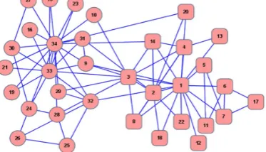
In some cases, the overlapping vertices in a graph are not so clearly, such as the “karate club” network of Zachary [17] which is shown in Fig. 2. AP can find the correct result, and choose vertex 1 as well as vertex 33 to be the exemplars of two clusters. In this network, there is no vertex

i

making r i( ,1)+a i( ,1)=r i( , 33)+a i( , 33). Then we look for the vertex

i

which makes the difference between r i( ,1)+a i( ,1) and

( , 33) ( , 33)

r i +a i smallest. Finally, vertex 3 has been picked up. This implies that for vertex 3, compared with other vertices, the difference of choosing vertex 1 or vertex 33 as its exemplar is insignificant. So vertex 3 may be an overlapping vertex. Choosing vertex 3 as an overlapping vertex is reasonable. In some algorithms, like GN and spectral partition, vertex 3 belongs to the cluster whose exemplar is vertex 33. While in MCL, with an appropriate parameter, vertex 3 is an overlapping vertex. We gain the conclusion that if only depend on the topology of the graph, it is difficult to decide which cluster vertex 3 belongs to. Vertex 3 could be an overlapping vertex.

AP can not identify the overlapping communities. However, the overlapping communities are ubiquitous in many real networks such as PPI networks, social networks as well as others. We can't use AP algorithm directly, but we can use the information AP gives us to identify the possible overlapping vertices. In this paper, we propose a new algorithm OAP based on AP, and this method could be used to detect the overlapping communities.

Fig. 2. Zachary’s karate club network. Square nodes and circle nodes represent the instructor’s faction and the administrator’s faction, respectively.

2) Identification of candidate overlapping vertices

We use the information AP offered to detect the candidate overlapping vertices. If a vertex

i

should be overlapped, then there must be several exemplars, and the difference of choosing which one as

i

’s exemplar is slight. To characterize the distinction of choosing different exemplars, a simple expression is given, stated

as distance i c k( , , )_i =r i c( , )_i +a i c( , ) ( ( , )_i − r i k +a i k( , )) . Here c_i represents the exemplar of vertex

i

found by AP.

k

is an exemplar of another cluster, and this cluster doesn’t include vertex

i

. distance i c k( , , )_i represents that for a vertex

i

, the difference between choosing

c

_i as its exemplar and choosing

k

as its exemplar.

We employ a parameter, threshold θ, in our OAP algorithm, which is a non-negative real number. If

( , , )i

distance i c k ≤θ , we consider that vertex

i

can

choose vertex

k

as its candidate exemplar, which means vertex

i

is chosen as a candidate overlapping vertex. We use θ to control the number of candidate overlapping vertices. With θ’s increasing, more and more candidate overlapping vertices will be found. The effect of parameter θ will be validated in the later experiments. The process of identifying candidate overlapping vertices is shown in algorithm 1:

Algorithm 1: Identifying candidate overlapping vertices algorithm

Input:

The adjacent matrix of graph

G

=

(

V

,

E

)

;

Output:

A hard partition of

V

, labeled as

{ }

1

m j _j

V ₌ , and

m

is the number of the communities we found;

A set of candidate overlapping vertices for each

V

_j,

labeled as CandidateSetj; Steps:

01 Calculate the similarity of every two vertices in

G

; 02 Run AP algorithm to get a hard partition of

V. Exemplars are stored in set

C

. We use

i

c

to represent the exemplar of vertex

i

;

03 Return

{ }

1

m

j _j

V

=

04 For each vertex

i

∈

V

do:

05 For each exemplar

j C

∈

do: 06 If distance i c j( , , )i ≤θ and j≠ci do:

07 CandidateSet_j =CandidateSet_j ∪{ }i ; 08 End If

09 End For 10 End For

11 Return

{

}

1

m j j

CandidateSet ₌

Using algorithm 1, each cluster found by AP has its own candidate overlapping vertices.

3) Filtering candidate overlapping vertices

For a vertex

i

, having an exemplar

c

satisfying ( , , )i

distance i c c ≤θ and

c c

≠

_i is only a necessary

than the same induced sub-graph without them.

In order to judge whether a graph is denser than another, we propose a density function of graph

( , )

G= V E as | | (| | 1)

| | (| | 1) / 2

G

E V

D

V V

− −

=

× − . Here

|

V

|

is the vertices number of

G

and

|

E

|

is the edges number of

G

. The biggest and only difference between graph density and ours is the factor

| | 1

V

−

in the numerator. The intuitive idea behind is that, similar to partition density given by Yong-Yeol Ann et al.[18], a tree is too sparse to be a significance function unit in PPI network becasue of the tree structure in ubiqutous in random graphs [19]. Another concept we introduce is vertex fitness. The fitness of an vertex

A

with respect to a sub-graph

G

,

f

_GA, is defined as the variation of the density of the sub-graph

G

with and without vertex A, i.e.

f

_GA

=

D

_{G+{ }A}

−

D

_{G−{ }A}

.

(5)

In equation (5), the symbol G+{ } (A G−{ })A indicates the sub-graph with vertex

A

inside (outside).

A filter strategy is suggested. Suppose graph

g

is a sub-graph and the candidate overlapping vertices of

g

is stored in a set CandidateSet. We find the vertex

i

in CandidateSet with the largest fitness and this candidate will be considered as a real overlapping vertex if

f

_gi

≥

0

. The pseudo code of filter strategy is stated in algorithm 2.

Algorithm 2: Filtering candidate overlapping vertices algorithm

Input:

The adjacent matrix of

G

=

(

V

,

E

)

; A cluster found by AP, labeled as

V

_j;

The set of candidate overlapping vertices for

V

_j , labeled as

CandidateSet

_j;

Output:

A cluster with overlapping vertices in it if necessary, labeled as

V

_j( )s .

Steps:

01

V

_j(s)

=

V

_j;

02 While

CandidateS

et

_j

≠

φ

do:

03 Calculate

D

_g.

//Graph g is the induced sub-graph of ( )s j

V ;

04 find the vertex

i

in CandidateSet_j with the largest fitness;

05 If

f

gi

≥

0

do

06

V

j( )s

=

V

j( )s

∪

{ }

i

;

07 else

08 Break; 09 End If

10 End While 11 Return

V

_j( )s

Using sub-algorithm 2, every cluster found by AP has been expanded to be an overlapping community if it is necessary.

4) Our algorithms OAP

Based on the analysis above, we propose a new method OAP to identify protein complexes in PPI networks. Our algorithms OAP are shown as follows:

OAP Algorithm Input: A PPI network

Output:

Protein complexes Steps:

1. Represent the PPI network by a graph

)

,

(

V

E

G

=

;

2. Run algorithm 1 to get a hard partition of the PPI network and identify candidate overlapping proteins for each module;

3. For each cluster

V

_j found by AP, its induced

sub-graph is labeled as graph

g

. If

D

_g

>

0

, run algorithm 2 to filter candidate overlapping proteins. 4. Return protein complexes.

The algorithm 1 consists of two parts. One part is AP, which is used to partition the PPI network, and the time complexity of it is

( )

2

N

Ο .

N

is the vertices number of

G

. Another part is used to identify candidate overlapping proteins for each community, and the time complexity of it is Ο

( )

Nm . Here

m

is the number of communities found by AP. Suppose each community has

n

candidate overlapping proteins on average. The time complexity of algorithm 2 is

( )

2

n m

Ο . Since

n

N

, the time complexity of algorithm 2 is lower than

( )

2

N

Ο . Therefore, the overall complexity of OAP is

2 2

( ) ( ) ( )

O N +O Nm +O n m which could be considered

as

( )

2

N

Ο .

We consider the protein complexes detected by OAP are more biological significant than those detected by AP. When using AP algorithm to clustering PPI network, we get a hard partition, and we regard each community in this partition as a complex. But in fact, a protein may belong to more than one complex, and those very sparse sub-graphs found by AP may biological insignificant. OAP get over these difficulties. It can filter those insignificant communities by comparing them with random graphs and identify overlapping communities by using the information AP gives us.

III.EXPERIMENTS AND RESULTS

In this section, we do some experiments to validate the efficiency of our method in identifying protein complexes in PPI networks.

A. Experimental data

In our experiments, we perform our OAP method on the yeast (S. cerevisiae) PPI network. The PPI network of budding yeast has been studied earlier in several works [6][9][20]. This data set is available in December 2007 release of the Database of Interaction Protein (DIP: http://dip.doe-mbi.ucla.edu/), which consists of 17,201 interactions between 4928 proteins (we delete isolated proteins and loops).

In order to evaluate our identified modules, a set of real complexes is selected as the benchmark [21]. This benchmark set consists of 428 protein complexes, from three sources: (I) MIPS [22], (II) Aloy et al. [23] and (III) SGD database [24] based on Gene Ontology (GO) annotations.

B. Evaluation criteria

Different criteria proposed by previous studies are used to evaluate clustering results for PPI networks ([25]Sylvain et al., 2006; [26]Chua et al., 2007; [27]Song et al., 2009). We use some of them to evaluate our experiment results.

1) Precision, Recall and F-measure

Before giving the definition of precision, recall and F-measure, we should define some other concepts first. The neighborhood affinity score between a real complex

b

in the benchmark and a predicted complex

p

is used to determine whether they match with each other or not, and is defined as

(

)

2

, b p

b p

V V

NA p b

V V

= × ∩

.

The neighborhood affinity score of a predicted complex vs. a benchmark complex is a measure of biological significance of the prediction. If

NA

( )

p

,

b

≥

ω

, then they are considered to be matching. In order to choose an appropriate

ω

that maximizes biological relevance of the predicted complexes without filtering away too many predictions, MCODE algorithm tested this parameter from 0 to 0.9 (in 0.1 increments). The experimental results demonstrate that a

ω

threshold of 0.2 to 0.3 can filter out most predicted complexes that have insignificant overlap with known complexes.

We set

ω

as 0.2 in this paper, which was the same threshold used in MCODE [28] and CoAch. Let

B

be the set of real complexes, it is the benchmark, and

P

be the set of clustering results.

N

_cpis the number of predicted complexes which match at least a real complex,

the mathematic expression is

{

| , , ( , )

}

cp

N = p p∈P b∃ ∈B NA p b ≥ω .

N

_cb is the number of real complexes which match at least a

predicted one, the mathematic expression is N_cb =

{

b b| ∈B p,∃ ∈P NA p b, ( , )≥ω

}

. Precision

and recall are defined as [26]:

| |

cp

N Precision

P

=

| |

cb

N Recall

B

=

F-measure which is the harmonic mean of precision and recall, defined as:

2 / ( )

F measure− = ×Precision Recall Precision Recall× + I t is used to evaluate the overall performance of the different techniques.

2) P-value

The P-value is often used to calculate the statistical and biological significance of a protein clusters, following the hyper-geometric distribution. It is the probability that a given set of proteins is enriched by a given functional group merely by chance [29]. Assume a cluster C of size

|

C

|

, with

k

proteins in a functional group

F

of size

|

F

|

. Also, assume the PPI network contains

|

V

|

proteins entirely. Then, the P-value is:

1

0

| | | | | |

| | 1

| |

| |

k

i

F V F

i C i

P value

V

C −

=

− −

− = −

⎛ ⎞⎛ ⎞ ⎜ ⎟⎜ ⎟ ⎝ ⎠⎝ ⎠

⎛ ⎞ ⎜ ⎟ ⎝ ⎠

∑

Known protein complexes have low P-value, because smaller P-value implies that the clustering is not random and is more biologically significant than the cluster with a higher P-value. In our experiments, those clusters whose P-value is bigger than 0.001 are considered to be insignificant.

C. Effect of the parameters

Our algorithm employs two parameters. The preference is the parameter we inherit from AP algorithm. It affects the number of modules. Here we only discuss how the parameter θ affects the results. The threshold

θ is a parameter which is used to control the number of candidate overlapping protein complexes. When θ is smaller than the exact value it should be, the clustering result is sensitive to θ, because we lose proteins that should be overlapped. When θ is larger than the exact value, the clustering result is not sensitive to θ, because we find enough candidate overlapping proteins and those not eligible were thrown off by the next step of our algorithm. But that doesn't mean we can set θ very big. Big θ will cause more candidates, and the more candidates we have, the more computing time we need.

In our experiments, we increase θ step by step. Here is the way we set θ: we construct two 1×N vectors,

1

V and 2V . N is the number of vertices. Here, The

i

th element in vector 1V is

r

(

i

,

c

_i

)

+

a

(

i

,

c

_i

)

.

j

is the vertex which minimize

))

,

(

)

,

(

(

)

,

(

)

,

(

i

c

a

i

c

r

i

j

a

i

j

r

_i

+

_i

−

+

and

j

≠

c

_i .

Then we calculate

1 1

( 1( ) 2( ))

N

i

base line V i V i

N =

=

∑

− . We

consider that θ won’t be bigger than the base line, otherwise there will be too much proteins chosen as candidate overlapping proteins.

We increase θ from zero to this base line by using 0.1×base line as the step length to study how threshold θ affects our results. The experimental results displayed in Fig. 3 and Fig. 4.

0 0.1 0.2 0.3 0.4 0.5 0.6 0.7 0.8 0.9 1 0

50 100 150 200 250

threshold

numbe

r of

ov

er

lapp

in

g prot

ei

ns

Fig. 3. The relationship of threshold θ and the number of overlapping proteins

0 0.1 0.2 0.3 0.4 0.5 0.6 0.7 0.8 0.9 1

0 50 100 150

threshold

num

be

r of

ov

e

rla

ppi

ng

p

rot

ei

n c

om

p

lexes

Fig. 4. The relationship of threshold θ and the number of overlapping protein complexes

When θ is smaller than 0.6×base line, increasing θ a little will cause an obvious increasement of the number of overlapping modules and the number of overlapping vertices. When threshold θ is bigger than 0.6×base line, these two numbers both increase slowly, until they keep stable finally. These experiments exactly validate our analysis of θ above. In the later experiments, the threshold θ we use is 0.6 times as big as the base line.

D. Comparisons with other algorithms

In this section, we compare the performance of our OAP with AP, MCL, CPM and CoAch. We apply the MCL algorithm to find protein complexes from the same DIP data. We set the inflation parameter in MCL to be 1.8, which makes the result have a best F-measure [25]. The performance of CPM, CoAch and AP is evaluated, too. We use the default setting of CoAch. While using CPM algorithm, we detect 3-cliques.

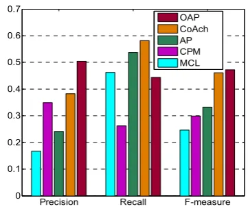
Precision Recall F-measure

0 0.1 0.2 0.3 0.4 0.5 0.6 0.7

OAP CoAch AP CPM MCL

Fig. 5. The comparisons between MCL, CPM, AP, and CoAch on precision, recall and f-measure

Fig. 5 displays the comparison result of OAP, CoAch, CPM, MCL and AP on evaluation criteria precision, recall and F-measure. The precision of our OAP is 50.4%, which is 200.7%, 44%, 109.3% and 32.0% higher than MCL, CPM, AP and CoAch respectively. This means our method can predict functional modules very accurately. The recall of our method is 44.4%, which is 26.7% and 17.3% lower than CoAch and AP. Because the number of protein complexes predicted by our algorithm is 232, which is far more less than that of CoAch and AP. The F-measure of our OAP is 47.2, which is 91.9%, 57.9%, 41.7% and 2.4% higher than MCL, CPM, AP and CoAch respectively. Our OAP still performs the best.

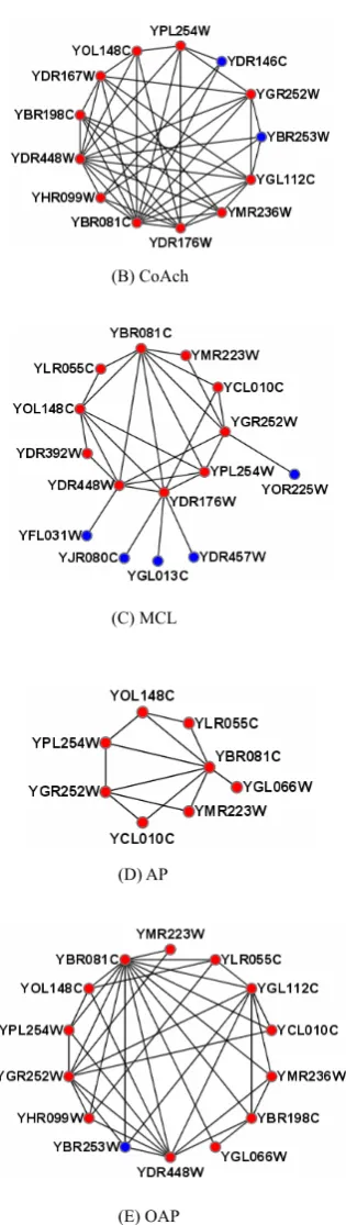
Fig. 6 illustrates an example, in which our predicted SAGA complex [30] can cover more proteins in the real SAGA complex. In this example, the real SAGA complex in the benchmark consists of 20 proteins. The complex predicted by our OAP method has 14 proteins and 13 of them are involved in the benchmark (in red color). The P-value is 1.95e-23. Meanwhile, CoAch method detect 13 proteins and manages to cover 11 proteins. The P-value is 4.49e-15. AP covers only 8 proteins of the real SAGA complex. The P-value is 1.33e-13. The complex predicted by MCL has 15 proteins and manages to cover 10 proteins. The P-value is 3.24e-15. MCODE algorithm can’t find a complex matches with SAGA complex, so it is not displayed in Fig. 6.

Fig. 6. The SAGA complex predicted by different methods. In fig.6, (A) shows the real SAGA complex in the benchmark, and (B-E) are the SAGA complex predicted by CoAch, MCL, AP and OAP respectively. For each predicted complex, the proteins in red color are involved in the real SAGA complex and those in blue color are not.

In table 1, the statistical significance of protein complexes predicted by various methods is displayed. A predicted complex is considered to be significant if its P-value is less than 0.001. The proportion of significant complexes over all predicted ones can be used to

evaluate the overall performance of various methods. Table 1 shows the comparison results based on this measure. From Table 1, it is easy to find out that our algorithm achieve the best performance.The proportion of our OAP is 93%, which is 146.0%, 36.2%, 69.1% and 11.5% higher than MCL, CPM, AP and CoAch respectively.

TABLE I.

STATISTICAL SIGNIFICANCE OF COMPLEXES PREDICTED BY VARIOUS METHODS

algorithm predicted protein Number of complexes

Number of Significant protein

complexes

Proportion (%)

OAP 232 216 93%

MCL 835 316 37.8%

AP 631 348 55%

CoAch 746 622 83.4%

CPM 240 164 68.3%

IV.CONCLUSION AND DISCUSSION

Identifying protein complexes within biological systems is necessary for comprehending the high-level organization of the cell. Some different protein complexes are overlapping because they have proteins in common. In this study, we develop a new algorithm based on AP algorithm to find overlapping protein complexes in PPI networks. This algorithm can be used for clustering undirected and weighted graphs. We identify 232 protein complexes in the yeast protein-protein interaction network. We validate these detected protein complexes by comparing them with the GO annotations and find out that most of the predict complexes are significant.

OAP inherits the good features of AP, that is, not have to know the number of the clusters in advance. It uses the iterative matrix of AP to search candidate overlapping vertices, and filter theses candidate vertices by a new graph density we suggested. These methods ensure that OAP can detect overlapping protein complexes and the results are all dense regions. OAP has achieved significantly higher F-measure than the competitive algorithms: AP, MCL, CPM and CoAch. Although We didn’t identify many protein complexes, our predicted complexes match very well with benchmark complexes. We believe our proposed method can provide more insights for future biological study.

ACKNOWLEDGMENT

This work was supported by the Key NSFC (No. 60933009), NSFC (No. 61072103 &No.61100157) and the Fundamental Research Funds for the Central Universities

(No.K50510030006&K50511030001&K5051106004)

REFERENCE

[1]L. H. Hartwell, J. J. Hopfield, S. Leibler and A. W. Murray, “From molecular to modular cell biology”, Nature 1999, 402:C47-C52.

[2]Tong, A.H., Drees, B., Nardelli, G., Bader, G.D., Brannetti, B., Castagnoli, L., Evangelista, M., Ferracuti, S., Nelson, B., Paoluzi, S. Quondam, M., Zucconi, A., Hogue, (B) CoAch

(C) MCL

(D) AP

combined experimental and computational strategy to define protein interaction networks for peptide recognition modules’, Science, Vol. 295, No. 5553, pp.321–324. [3]Tornow, S. and Mewes, H. (2003) ‘Functional modules by

relating protein interaction networks and gene expression’, Nucleic Acid Research, Vol. 31, No. 21, pp. 6283-6289. [4]Spirin, V. and Mirny, L.A. (2003) ‘Protein complexes and

functional modules in molecular networks’, Proc. Natl. Acad. Sci., Vol. 100, No. 21, pp.12123-12128.

[5]Palla, G., Derenyi, I., Farkas, I. and Vicsek, T. (2005) ‘Uncovering the overlapping community structure of complex networks in nature and society’, Nature, Vol. 435, No. 7043, pp.814-818

[6]Wu, M., Li, X., Kwoh, C.K. and Ng, S.K. (2009) ‘A core-attachment based method to detect protein complexes in PPI networks’, BMC Bioinformatics , Vol. 10, No.1, p.169.

[7]Girvan, M. and Newman, M.E. (2002) ‘Community structure in social and biological networks’,Proc. Natl. Acad. Sci., Vol. 99, No.12, pp.7821-7826

[8]Newman, M.E. (2004) ‘Fast algorithm for detecting community structure in networks’, Phys. Rev. E , Vol. 69, No.1, p.066133.

[9]Arnau, V., Mars, S. and Marin, I. (2005) ‘Iterative cluster analysis of protein interaction data’,Bioinformatics, Vol. 21, No. 3, pp.364–378.

[10] Dongen, S. V. (2000) ‘Graph Clustering by Flow Simulation’, University of Utrecht, Netherlands.

[11] Steve, G. (2007) ‘An algorithm to find overlapping community structure in networks’, In Proceedings of the 11th European Conference on Principles and Practice of Knowledge Discovery in Databases (PKDD), pp. 91-102. [12] Shen, H. W., Cheng, X., Cai, K. and Hu, M. (2009)

‘Detect overlapping and hierarchical community structure in networks’, Physica A, Vol. 388, No. 1, pp.1706-1712. [13] Wang, Y. and Gao, L., (2010) ‘An improved AP algorithm

for identifying overlapping functional modules in protein-protein interaction networks’, IEEE International Conference on Signal Processing (ICSP10) Proceedings, pp. 1809-1812.

[14] Frey, B.J. and Dueck, D. (2007) ‘Clustering by passing messages between data points’, Science, Vol. 315, No. 5814, pp.972-976.

[15] James, V. (2009) ‘Markov clustering versus affinity propagation for the partitioning of protein interaction graphs’, BMC Bioinformatics, Vol. 10, No. 1, p.99 [16] Jaccard, P., Bulletin de la Soci′et′e Vaudoise des (1901)

‘Distribution de la flore alpine dans le basin des Dranses et dans quelques régions voisines’, Sciences Naturelles Vol.37, No. 547, pp.241-272

[17] Zachary, W. W. (1977) ‘An information flow model for conflict and fission in small groups’, Journal of Anthropological Research, Vol. 33, No. 1, pp.452-473 [18] Ahn, Y. Y., Bagrow, J. P. and Lehmann, S. (2010) ‘Link

communities reveal multiscale complexity in networks’, Nature 2010 466:761

[19] Bollobas, B. (2001) ‘Random graphs’, Academic Press, London

[20] Asur, S., Ucar, D. and Parthasarathy, S. (2007) ‘An ensemble framework for clusteringprotein-protein interaction networks’, Bioinformatics, Vol. 23, No. 13, pp. 29–40.

[21] Friedel, C.C., Krumsiek, J. and Zimmer, R. (2009) ‘Boostrapping the interactome: unsupervised identification of protein complexes in yeast’, Journal of Computational Biology, Vol. 16, No. 8, pp.1-17.

[22] Mewes, H.W., Amid, C., Arnold, R., Frishman, D., Guldener, U., Mannhaupt, G., Munsterkotter, M., Pagel, P., Strack, N., Stumpflen, V., Warfsmann, J. and Ruepp, A. (2004) ‘MIPS: analysis and annotation of proteins from whole genomes’. Nucleic Acids Res., Vol. 32, Database issue, pp.41-44.

[23]Aloy, P., Bottcher, B., Ceulemans, H., Leutwein, C., Mellwig, C., Fischer, S., Gavin, A.C., Bork, P., Superti-Furga, G. and Serrano, L. (2004) ‘Structurebased assembly of protein complexes in yeast’, Science, Vol. 303, No. 5666, pp.2026-2029.

[24]Dwight, S.S., Harris. M.A., Dolinski, K., Ball, C.A., Binkley, G., Christie, K.R., Fisk, D.G., Issel-Tarver, L., Schroeder, M., Sherlock, G., Sethuraman, A., Weng, S., Botstein, D. and Cherry, J.M. (2002) ‘Saccharomyces Genome Database provides secondary gene annotation using the Gene Ontology’, Nucleic Acids Res., Vol. 30, No. 1., pp. 69-72.

[25]Sylvain, B. and Jacques, V. H. (2006) ‘Evaluation of clustering algorithms for protein-protein interaction networks’, BMC Bioinfomatics, Vol. 7, No. 1, p.488. [26]Chua, H.N., Ning, K., Sung, W.K., Leong, H.W. and

Wong, L(2007) ‘Using indirect protein-protein interactions for protein complex prediction’, CSB, pp.97-109.

[27]Song, J.M. and Mona, S. (2009)‘How and When should interaction-derived clusters be used to predict functional modules and protein function?’, Bioinformatics, Vol. 25, No. 23, pp. 3143-3150.

[28]Bader, G.D. and Hogue, C.W. (2003) ‘An automated method for finding molecular complexes in large protein interaction networks’, BMC Bioinformatics, Vol. 4, No. 1, p.2.

[29]King, A.D., Przulj, N. and Jurisica, I. (2004) ‘Protein complex prediction via cost-based clustering’, Bioinformatics, Vol. 20, No. 17, pp.3013–3020.

[30]Grant, P.A., Schieltz, D., Pray-Grant, M.G., Steger, D.J., Reese, J.C., Yates, J.R. and Workman, J.L. (1998) ‘A subset of TAF(II)s are integral components of the SAGA complex required for nucleosome acetylation and transcriptional stimulation’, Cell, Vol. 94, No.1, pp.45-53.

Yu Wang is currently a PhD student at the School of Computer Science and Technology of Xidian University Xi’an, China. She received her Master of Management from the School of Economics and Management of Xidian University (2006) and her Bachelor of Management from School of Economics and Management of Xidian University (2003). Her

research interests include bioinformatics, data mining, and complex network.