ISSN (e): 2250-3021, ISSN (p): 2278-8719 Vol. 08, Issue 11 (November. 2018), ||V (I) || PP 01-10
On three Parameter Weighted Quasi Akash Distribution:
Properties and Applications
Anwar Hassan, Gulzar Ahmad Shalbaf and Bilal Ahmad Para
Department of Statistics, University of Kashmir, Srinagar (J&K), IndiaCorresponding Author:Anwar Hassan
Abstract: In this paper, we have introduced a weighted model of the Quasi Akash Distribution and the weight
function considered here is
W
x
x
c, where the weight parameter isc
. We have investigated different characteristics as well as the structural properties of the Weighted Quasi Akash Distribution (WQAD). We have also derived the Moment Generating Function, Characteristic Function, Reliability Function and Hazard Rate function of the introduced model. Finally model has been examined with real life data.Keywords: Weighted Quasi Akash Distribution, Weighting Technique, Structural Properties and Maximum Likelihood Estimation.
--- Date of Submission: 08-11-2018 Date of acceptance: 22-11-2018 ---
I. INTRODUCTION
A two parameter Quasi Akash distribution (QAD) having parameters
and
introduced by Shanker (2016) is defined by its probability density function (pdf)x
e
x
x
f
(
)
2
)
,
;
(
22
0
,
0
,
0
x
(1.1)The corresponding cdf of (1.1) is given by
0
,
0
,
0
,
2
)
2
(
1
1
)
,
;
(
x
e
x
x
x
F
x (1.2)Shanker et al. (2016) have a detailed study on applications of QAD for modeling life time data.
II. WEIGHTED QUASI AKASH DISTRIBUTION (WQAD)
,
0
x
x
w
E
x
f
x
W
x
f
w ,where
w
(x
)
be a non-negative weight function andE
w
x
w
x
f
x
dx
.In this paper, we have considered the weight function as
w
x
x
c to obtain the weighted quasi Akash model. The probability density of weighted Quasi Akash distribution is given as:
c cw
x
E
x
f
x
c
x
f
,
,
,
,
,
,
,
))
2
)(
1
(
(
!
)
(
,
,
,
2 )
2 (
c
c
c
e
x
x
c
x
f
x c
c
w
0
,
0
,
0
,
0
c
x
(2.1)where
)
2
(
)
2
)(
1
(
!
c
c
c
c
c
x
E
.The corresponding cdf of weighted Quasi Akash Distribution (WQAD) is obtained as
x w
w
x
c
f
x
c
dx
F
0
)
,
,
;
(
)
,
,
;
(
x c c x
dx
c
c
c
e
x
x
0
2 )
2 (
))
2
)(
1
(
(
!
)
(
, put
x
t
,
dx
dt
,x
t
x
x
and
t
x
as
0
,
0
,
, after simplification,
))
,
3
(
)
,
1
(
(
))
2
)(
1
(
(
!
1
)
,
,
;
(
c
x
c
x
c
c
c
c
x
F
w
(2.2)
x
0
,
0
,
c
0
,
0
Where c,
and
are positive parameters and
s
x
xt
se
tdt
0 1
,
is a lower incomplete gammafunction.
III.SPECIAL CASES OF WQAD.
Case i: If we put
c
0
, then weighted Quasi Akash distribution (2.1) reduces to Quasi Akash distribution with probability density function as:x
e
x
x
f
(
)
2
)
,
;
(
22
x
0
,
0
,
0
Case ii: if we put c=0 and
, then weighted Quasi Akash distribution (2.1) reduces to Akash distribution with probability density function as:.
0
,
0
;
)
1
(
2
)
;
(
22 3
x
e
x
x
f
xCase iii: If we put c=
0, then weighted quasi Akash distribution reduces to gamma distribution. i.e;.
0
,
0
;
2
)
;
(
23
x
e
x
x
f
xIV.Moments and Related Properties:
4.1 Moment Generating Function (MGF): The moment generating function of WQAD (2.1) is as follows
0
(
)
)
(
)
(
t
E
e
e
f
x
dx
M
wx t x
t X
0
2 2
)]
2
)(
1
(
[
!
)
(
]
[
dx
e
c
c
c
x
x
e
xc c x
t
1
)(
2
)
(
]
)
2
(
)
1
(
[
]
)
3
(
)
2
(
[
)
1
(
1
c
c
c
c
c
[
(
1
)
(
2
)
]
]
)
4
(
)
3
(
)[
2
(
)
1
(
2 2
c
c
c
c
c
c
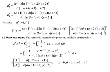
Variance
2
(
1
)
22 2
)]
2
(
)
1
(
[
)
3
)(
2
(
[
)
1
(
]
)
2
(
)
1
(
[
]
)
4
(
)
3
(
)[
2
(
)
1
(
)
(
c
c
c
c
c
c
c
c
c
c
c
x
V
4.2 Harmonic mean: The harmonic mean for the proposed model is computed as
dx
c
x
f
x
X
E
M
H
.
1
1
w(
;
,
,
)
0
x
d
e
c
c
c
x
x
x
x c c
)]
2
)(
1
(
[
!
)
(
]
[
1
2 20
,
]
)
2
(
)
1
(
[
]
)
1
(
[
1
c
c
c
c
c
X
E
x
0
,
0
,
0
,
c
0
.
V. RELIABILITY, HAZARD AND REVERSE HAZARD FUNCTIONS:
In this, we have obtained the reliability, hazard rate, reverse hazard rate of the proposed weighted Quasi Akash distribution.
5.1 Reliability function
R
( x
)
:The reliability function is defined as the probability that a system survives beyond a specified time .It can be computed as complement of the cumulative distribution function of the model. The reliability function or the survival function of weighted Quasi Akash distribution is computed as
)
(
1
)
,
,
,
(
x
c
F
x
R
w
w
)]
2
)(
1
(
[
!
)
(
]
)
,
3
(
)
,
1
(
[
1
c
c
c
x
c
x
c
(5.1.1)
x
0
,
0
,
c
0
,
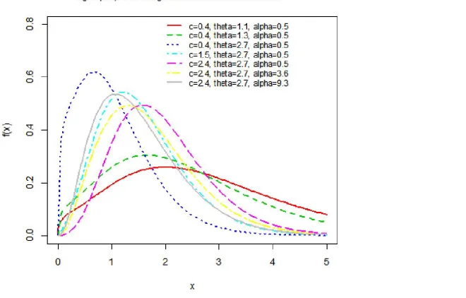
The graphical representation of the reliability function for the weighted Quasi Akash distribution is shown in fig. 3.
5.2 Hazard function:
The hazard function is also known as hazard rate ,defined as the instantaneous failure rate or force of mortality
and is given as:
]
)
,
3
(
)
),
(
[
)]
2
(
)
1
(
[
)!
(
)
(
)
,
,
,
(
)
,
,
,
(
.
2 2x
c
x
c
c
c
c
e
x
x
c
x
R
c
x
f
R
H
x c c w w
5.3 Reverse Hazard Rate:
The reverse hazard rate of weighted Quasi Akash distribution is given as
(
1
,
)
(
3
,
)
VI.ORDER STATISTICS
Let
X
(1),
X
(2),...,
X
(n) be the ordered statistics of the random sampleX
1,
X
2,...,
X
ndrawn from the continuous distribution with cumulative distribution functionF
X( x
)
and probability density functionf
X( x
)
,then the probability density function of
r
thorder statisticsX
(r)is given by:n
r
x
F
x
F
x
f
r
n
r
n
c
X
f
r n rr
X
(
)
[
(
)]
[
1
(
)
]
,
1
,
2
,
3
,....,
)!
(
!
)
1
(
!
)
(
)
,
,
;
(
1)
(
Using the equations (2.1) and (2.2), the probability density function of rth order statistics of weighted Quasi Akash distribution is given by:
r n
r x
c c
r w
c
c
c
x
c
x
c
c
c
c
x
c
x
c
c
c
c
e
x
x
r
n
r
n
c
X
f
)]
2
)(
1
(
[
)!
(
,
3
(
)
,
1
(
1
]
)
2
)(
1
(
[
!
)
(
)
,
3
(
)
,
1
(
]
)
2
(
)
1
(
[
!
)
(
)
(
)!
(
!
)
1
(
!
)
(
)
,
,
;
(
1 2
2
) (
1 2 2 ) (
]
)
2
)(
1
(
[
!
)
(
)
,
3
(
)
,
1
(
]
)
2
(
)
1
(
[
!
)
(
)
(
)
,
,
;
(
n x c c n wc
c
c
x
c
x
c
c
c
c
e
x
x
n
c
X
f
VII. RANDOM NUMBER GENERATION FROM WQLD
In this section, we discuss the random number generation from WQAD. We generally employ Inverse cdf Method for the generation of random numbers from a particular distribution. In this method the random numbers from a particular distribution are generated by solving the equation obtained on equating the cdf of a distribution to a number u. The number u is itself being generated from
U
0
,
1
. Thus following the same steps for the purpose of random number generation from the WQAD, we will proceed as( ; , , ) = .
Where ( ; , , ) is the cdf of WQAD and u is the random number generated from uniform distribution i.e.,
0
,
1
U
.!( ( )( )) ( + 1, ) + ( + 3, ) = (7.1)
On solving the equation (7.1) for
x
, we will obtain the required random number from the WQAD. Main problem, which is being faced while using this method of generating the random numbers is to solve the equations which are usually complex and complicated. In order to overcome such hindrance, we use softwares like MATLAB, Mathematica, SAS or R for solving such a complex equation.VIII. METHOD OF MAXIMUM LIKELIHOOD ESTIMATION OF WEIGHTED QUASI
AKASH DISTRIBUTION
This is one of the most useful method for estimating the different parameters of the distribution. Let
n
X
X
X
X
1,
2,
3...
be the random sample of size n drawn from weighted Quasi Akash distribution, then thelikelihood function of weighted Quasi Akash distribution is given as:
n i n i x c cc
c
c
e
x
x
c
x
f
c
x
L
1 1 2 ) 2 ())
2
)(
1
(
(
!
)
(
)
,
,
;
(
,
,
|
The log likelihood function becomes:).
2
)(
1
log(
)!
(
log
)
(
log
log
log
)
2
(
log
log
1 2 1
c
c
n
c
n
x
x
c
n
x
c
L
n i i i n ii
(8.1)
Differentiating the log-likelihood function with respect to θ,
andc
.This is done by partially differentiate (8.1) with respect to θ,
andc
and equating the result to zero, we obtain the following normal equations,0
)
(
_
)
2
(
log
1 2 1 1 2
n i i n i i n i ix
x
x
c
n
L
(8.2)0
)
(
log
1 2
n i ix
n
L
(8.3)By solving equations (8.1), (8.2) and (8.3), the maximum likelihood estimators of the parameters of the weighted Quasi Akash distribution are obtained using the numerical methods like Newton Raphson method. We can compute the maximized unrestricted and restricted log likelihoods to construct the likelihood ratio (LR) statistics for testing the significance of weighted parameter of the proposed model. For example, we can use LR test to check whether the fitted weighted Quasi Akash distribution for a given data set is statistically “superior” to the fitted Quasi Akash distribution. In any case, hypothesis tests of the type
H
0:
0 versus0 1
:
H
can be performed using LR statistics. In this case, the LR statistic for testing H0 versus H1 is))
ˆ
(
)
ˆ
(
(
2
0
L
L
where
ˆ
and
ˆ
0are the MLEs under H1 and H0. The statistic
is asymptotically
n
as
(
) distributed as
k2, with k degrees of freedom which is equal to the difference in dimensionalityof
ˆ
and
ˆ
0. H0 will be rejected if the LR-test p-value is <0.05 at 95% confidence level.8.1 Simulation Study of ML estimators of WQAD
The performance of ML estimators of WQAD for different sample sizes (n=25,75,100,150,300,500) has been discussed in this section. Inverse cdf technique for data simulation for WQAD using R software has been employed. The process was repeated 500 times for calculation of bias, variance and MSE as given values in table 1. For two random parameter combinations of WQAD, we observe decreasing trend in average bias, variance and MSE as we increase the sample size. Hence, the performance of ML estimators is quite well, consistent in case of WQAD.
Table 1: Simulation Study of ML estimators for weighted Quasi Akash Distribution
Parameter n = 0.5, = 0.7, = 0.8 = 1.6, = 0.9, = 1.9
Bias Variance MSE Bias Variance MSE
25
0.834899 0.211666 0.908722 0.994085 0.441057 1.429262
0.987854 0.121255 1.097111 1.02354 0.23541 1.283044
0.099080 0.013196 0.023013 0.222888 0.020859 0.070538
75
0.683829 0.120782 0.588404 0.451215 0.226023 0.429618
0.865970 0.116740 0.866644 0.768745 0.511739 1.102708
0.086580 0.012579 0.020075 0.211215 0.003211 0.047823
100
0.551480 0.096800 0.400930 0.33123 0.092468 0.202181
0.741917 0.084289 0.634729 0.623027 0.198717 0.586879
0.053770 0.014081 0.016972 0.152203 0.003214 0.02638
150
0.449400 0.051392 0.253352 0.272492 0.009101 0.083353
0.681953 0.043215 0.508275 0.4114 0.111809 0.281058
0.060080 0.005101 0.008711 0.154116 0.004113 0.027865
300
0.288480 0.007064 0.090285 0.11823 0.002912 0.01689
0.644068 0.011107 0.425930 0.201545 0.026483 0.067103
0.066488 0.001229 0.005650 0.110114 0.004106 0.016231
500
0.185541 0.000280 0.034705 0.09878 0.000136 0.009894
0.522348 0.001699 0.274546 0.135097 0.001537 0.019788large samples. Even though in small samples, the AIC, AICC, BIC and Negative Loglikelihood values are also minimum in case of Weighted model but the likelihood ratio test reveals that the role of weighted parameter exhibits a highly significant role in case of large samples only. LR statistic for testing H0 versus H1 is
))
ˆ
(
)
ˆ
(
(
2
0
L
L
, where
ˆ
and
ˆ
0are the MLEs under H1 and H0. The statistic
is asymptotically
n
as
(
) distributed as
k2, with k degrees of freedom which is equal to the difference in dimensionalityof
ˆ
and
ˆ
0. H0 will be rejected if the LR-test p-value is <0.01 (or LR Statistic value >6.635) at 99%confidence level
Table 2: Comparison of WQAD and QAD Based On Simulated Data.
̂ = 0.5 , = 1.5 , = 1.0 Parameter Estimates Likelihood Ratio Statistic Criterion WQAD QAD
Sample
Size (n) WQAD QAD -logL 14.55305 14.57047
10
̂ =0.168 (0.931) =0.325 (0.668) =1.46 (0.497)
=0.024 (0.321)
=1.398 (0.289) 0.0348 AIC 35.10609 33.14094
AICC 39.10609 34.85522 BIC 36.01385 33.74611 -logL 48.08946 48.83002
25
̂ =0.991 (0.781) = 2.79 (1.012) =1.07 (0.233)
=0.307 (0.427)
=0.896 (0.134) 1.4811 AIC 102.1789 101.66
AICC 103.3218 102.2055 BIC 105.8355 104.0978 -logL 197.5296 200.0704
100
̂ =1.135 (0.321) =10.96 (2.354) = 0.959 (0.13)
=0.222 (0.191)
=0.926 (0.071) 5.0815 AIC 401.0592 404.1408
AICC 401.3092 404.2645 BIC 408.8747 409.3511 -logL 574.8448 580.1859
300
̂ =0.858 (0.246) =5.326 (1.966) =1.001 (0.084)
=0.428 (0.185)
=0.934 (0.052) 10.682 AIC 1155.69 1164.372
AICC 1155.771 1164.412 BIC 1166.801 1171.779 -logL 1951.565 1960.477
1000
̂ =0.781 (0.156) =2.469 (0.991) =1.031 (0.034)
=0.288 (0.059)
=0.921 (0.021) 17.825 AIC 3909.129 3924.954
AICC 3909.153 3924.966 BIC 3923.852 3934.77
Table 3: Model Comparison Based On Simulated Data from WQLD.
̂ = 1.2, = 0.2, = 1.5 Parameter Estimates Likelihood Ratio Statistic Criterion WQLD QLD
Sample
Size (n) WQLD QED -logL 17.22829 17.82711
10
̂ =1.33 (0.80) =0.001 (0.89) =1.41 (0.45)
=0.102 (0.561)
=0.96 (0.127) 1.19763 AIC 40.45658 39.65422
AICC 44.45658 41.3685 BIC 41.36433 40.25939 -logL 42.26757 44.51678
25
̂ =2.05 (0.64) =0.001 (0.87) =1.59 (0.33)
=0.112 (0.458)
=0.931 (0.08) 4.4984 AIC 90.53513 93.03356
-logL 166.978 173.1069
100
̂ =2.04 (0.851) =0.798 (0.79) =1.64 (0.251)
=0.101 (0.171)
=0.989 (0.069) 12.2578 AIC 339.956 350.2139
AICC 340.206 350.3376 BIC 347.7715 355.4242 -logL 511.7328 522.3951
300
̂ =1.924 (0.641) =1.612 (0.68) =1.59 (0.203)
=0.10 (0.269)
=1.019 (0.07) 21.3244 AIC 1029.466 1048.79
AICC 1029.547 1048.831 BIC 1040.577 1056.198 -logL 1633.577 1679.299
1000
̂ =1.122 (0.25) =0.028 (0.09) =1.51 (0.08)
=0.11 (0.1310)
=1.07 (0.02) 91.4451 AIC 3273.153 3362.598
AICC 3273.177 3362.61 BIC 3287.876 3372.414
X. APPLICATIONS OF WEIGHTED QUASI AKASH DISTRIBUTIONS
Here we analyse the data set given in table 4, studied by Xu et al. (2003) and it represents the time to failure (103h) of turbocharger of one type of engine.
Table 4: The time to failure of turbocharger data (n = 40) studied by Xu et al. (2003). 1.6 3.5 4.8 5.4 6.0 6.5 7 7.3 7.7 8 8.4 2 3.9 5 5.6 6.1 6.5 7.1 7.3 7.8 8.1 8.4 2.6 4.5 5.1 5.8 6.3 6.7 7.3 7.7 7.9 8.3 8.5 3 4.6 5.3 6 8.7 8.8 9
In order to compare the performance of weighted Quasi Akash Distribution vz Quasi Akash Distribution, we employ AIC (Akaike information criterion by Akaike (1976)), AICC (corrected Akaike information criterion) and BIC (Bayesian information criterion given by Schwarz (1987)) criterion. The better distribution corresponds to minimum of AIC, AICC and BIC values. The generic formulas for AIC, AICC and BIC are given as,
AIC = 2k-2logL AICC = AIC+
1
)
1
(
2
k
n
k
k
and BIC = k logn-2logL
where k is the number of parameters in the statistical model, n is the sample size and -logL is the maximized value of the log-likelihood function under the considered model. R software was used to analyse the failure of turbocharger data (n = 40) studied by Xu et al. (2003). From table 5, it is clear that Weighted Quasi Akash Distribution (WQAD) has the lesser AIC, AICC, -logL and BIC values as compared to Quasi Akash Distribution. Hence we can conclude that the Weighted Quasi Akash distribution leads to a better fit than the Quasi Akash distribution. We also test the significance of weighted parameter c with the help of Kolmogorov Smirnov test. The p-value for WQAD is greater than 0.05, which signifies that data come from WQAD.
Table 5: ML estimates, -logL, AIC, AICC, BIC, Kolmogorov Smirnov statistic and KS p-values calculation for time to failure of turbocharger data (n = 40) studied by Xu et al. (2003). Model ML Estimates -logL AIC AICC BIC KS-Distance P-Value
Weighted Quasi Akash
7
.
11
ˆ
35
.
1
ˆ
93
.
5
ˆ
c
parameter Quasi Akash distribution as the base distribution. Some mathematical properties along with reliability measures are discussed. The hazard rate function and reliability behavior of the weighted Quasi Akash distribution exhibits that subject distribution can be used as a lifetime model.
REFERENCES
[1]. Akaike, H. (1976). A new look at the statistical model identification. IEEE Trans. Autom.Control , 19 , 716–723.
[2]. Ayesha, A. (2017). Size Biased Lindley Distribution and Its Properties a Special Case of Weighted Distribution. Applied Mathematics, 08(06), 808-819.
[3]. Buckland, W. R., & Cox, D. R. (1964). Renewal Theory. Biometrika, 51(1/2), 290. doi:10.2307/2334228 [4]. Fisher, R.A. (1934). The effects of methods of ascertainment upon the estimation of frequencies. Ann.
Eugenics, 6, 13-25.
[5]. Jing (2010) Weighted Inverse Weibull and Beta-Inverse Weibull Distribution, Georgia Southern University Digital Commons@Georgia Southern.
[6]. Patil, G. P., & Rao, C. R. (1978). Weighted Distributions and Size-Biased Sampling with Applications to Wildlife Populations and Human Families. Biometrics, 34(2), 179. doi:10.2307/2530008
[7]. Rao, C. R. (1965). On discrete distributions arising out of method of ascertainment, in classical and Contagious Discrete, G.P. Patil .ed ;Pergamon Press and Statistical publishing Society, Calcutta, pp-320-332.
[8]. Schwarz, G. (1987). Estimating the dimension of a model. Ann. Stat., 5, 461–464. [9]. Shanker, R. (2016). A Quasi Akash Distribution. ASR, 30 (1), 135-159.
[10]. Shanker, R., & Shukla, K. K. A Generalized Size-Biased Poisson-Lindley Distribution and Its Applications to Model Size Distribution of Freely-Forming Small Group. Journal of Scientific Research, 10(2), 145, (2018)
[11]. Taillie, C., Patil, G.P. and Hennemuth, R. (1995). Modelling and analysis of recruitment distributions, Ecological and Environmental Statistics, 2(4), 315-329.
[12]. Warren, W. G. (1975). Statistical Distributions in Forestry and Forest Products Research. A Modern Course on Statistical Distributions in Scientific Work, 369-384. doi:10.1007/978-94-010-1845-6_27 [13]. Xu, K., Xie, M., Tang, L.C. and Ho, S.L. (2003). Application of neural networks in forecasting engine
systems reliability, Applied Soft Computing, 2 (4), 255-268.