C. L. BATCHELER1 and D. G. CRAIB2
1. Forest Research Institute, New Zealand Forest Service, P.O. Box 31-011, Christchurch, New Zealand. 2. New Zealand Forest Service, P.O. Box 138, Hokitika, New Zealand.
83
A
VARIABLE AREA PLOT METHOD OF ASSESSMENT OF
FOREST CONDITION AND TREND
Summary: The properties of a variable area sampling technique, by which the observer varies the search-radius to obtain approximately a prescribed number of woody plants in each tier measured, were determined by (i) comparison of fixed area and variable area sampling of a computer-mapped shrub population; (ii) comparison of results from fixed area and variable area sampling of woody plants exceeding about 2m height in a rata-kamahi forest; (iii) two variable area surveys of woody plants exceeding 30cm height in a beech forest.
Variable area sampling gave unbiased estimates of crown area and plant density in the computer-mapped population. These were as precise as estimates obtained by fixed area sampling when sampling intensities were equal. For the same number of plots, 20 m x 20 m fixed area sampling of density and basal area in rata-kamahi forest was more precise than variable area sampling in plots containing 30 stems per plot, but in terms of sampling intensity and time, variable area sampling was more efficient. Both sampling methods gave similar stem diameter frequency patterns. Two surveys of beech forest, conducted 11 years apart, showed that with about 70-80 single-tier plots, differences in basal area of about 15% can be detected using the variable area plot method.
Variable area sampling is robust and suitable for ecological surveys of New Zealand's indigenous forests. Keywords: vegetation sampling, unbiased estimator, accuracy, precision, basal area, diameter distribution.
Introduction
The design of sampling procedures for surveys of protection forests is complicated by the need to estimate a wide range of parameters of forest trend, condition and animal effects during a single, logistically manageable operation.
Assessment of trend and condition of the vegetation is a complex problem: 'trend' is an unambiguous concept by which change is measured or otherwise assessed; but 'condition' may be judged in many terms, such as the quality of a habitat for sustaining a harvest of possum skins, for birds, rare plants, or its semblance to a pristine state. For this paper, we define it as a measure of whether the forest is maintaining itself structurally and physiognomically, and so is able to anchor the soil mantle and maintain the premitive land-form (Batcheler and Wardle, 1976). For this purpose, the main indices are species composition, plant age distributions (as deduced from diameter distribution), and basal area as an index of the degree of
occupation of the site.
Most quantitative inventories of watershed forests have used plots of fixed area (FA plots) (Holloway and Wendelken, 1957; Allen and McLennan, 1983). Currently, the "standard" plot used is 20 m x 20 m (Allen and McLennan, 1983), which evolved from the minimal area concept of Greig-Smith (1957) and the experience of Wardle (1970:534) with splot-less
(syn. non-area reconnaissance) sampling of beech (Nothofagus) forests.
However, use of a single sampling unit has severe practical problems. Intricate mosaics within
protection forests are frequent, and thickets containing several thousand stems per hectare are often interspersed with tall forest containing less than 200 stems per hectare. In subalpine scrub, inventory of a 20 m x 20 m plot can take more than one day for a four-man party. In tall forest it can take about two hours. Although smaller plots have been used to measure thickets in some surveys, use of a limited number of plot sizes is only a partial attempt to optimize sampling of a continuum of possible vegetation structures and densities.
In an attempt to resolve the problem, Jane (1982) outlined a "constant count" method for measuring woody plants with definable stems. A prescribed number of stems (m) are sampled in each defined tier (e.g., trees, saplings, seedlings) and the radius of the plot which exactly includes that mth individual is recorded. He suggested a target count of about 20 plants for each tier. Density of the tier is then estimated as:
D = (n - l)m.∑ (l/r2)/(n2.π)
where n is the number of samples, m is the constant count number, and r is variable radius (Eberhardt, 1967).
However, there are practical difficulties in identifying the mth individual. The procedure involves careful spiral sweeps around the sample point, measuring and tallying plants until the target number is reached. Identifying the mth individual frequently involves time-consuming rechecking of measurements near the boundary, and amendment of the records.
A simpler approach to flexible plot sampling is to judge the radius from the plot centre which should include the target count within the defined tier, and to adhere to that radius whether or not the target count is achieved. We call this method variable area (V A) sampling. Unlike Jane's procedure, it is not an exact "constant count" method and although it has much in common with "point-sampling" as used in forestry (e.g. Grosenbaugh and Stover, 1957), point sampling is usually associated with angle gauge estimation of basal area.
This paper discusses accuracy and precision of V A sampling of a computer-mapped population, the comparative precision and efficiency of FA and V A sampling in a complex rata-kamahi (Metrosideros umbellata - Weinmannia racemosa) forest, and the degree of basal area changes detectable using VA sampling in a relatively simple montane beech forest.
Methods
Throughout the paper, sampling errors of means are given as ± 95% PLE (probable limit of error, equivalent to half the confidence interval), calculated from tS/√N, where t = Student's t, S is standard deviation, and N is number of samples. Where appropriate, CV (coefficient of variation), = S/mean, or CV%, are used.
1. Computer-mapped population
Lyon (1968) measured the X- Y co-ordinates, height and crown dimensions of 3953 bitterbrush (Purshia tridentata) and associated plants in a 500 x 700 ft area in Montana, USA. Our study uses Lyon's data for a 1.3 ha (350 ft x 400 ft) sub-area containing 1535 plants (L. J. Lyon, pers. comm.). The X- Y co-ordinates and the maximum and minimum crown diameters of these plants were stored on a computer and sampled from pseudo-random co-ordinates by FA and V A plots. Edge effects were obviated by using the computer to construct four contiguous "copies" of the population and by confining sampling to a central rectangle of the same dimensions as the original surface. The distribution of the population
was assessed by sampling with 400 circular random plots containing averages of 2.5 and 10 plants per plot. The comparative accuracy of FA and V A sampling was determined by using several sampling runs of 2 to 141 circular random plots expected to contain averages of 8, 16, and 32 plants per plot (m). Appropriate sizes (a) of the FA plots were determined from
a = (m.total area)/1535
The program was devised to complete the FA search at each sample point, and then use the count of plants (c) as a guide to the required VA plot area (a' ) needed at that locus:
a' = a.m/c
This procedure resulted in a positive bias of about 11 % when the area of VA plots was not restricted, because clusters of plants were occasionally
"captured" just within V A boundaries centred on loci occupied by a low density phase of the population. Therefore, in the experiments reported here, areas were iteratively reduced by 10% decrements when the tally exceeded the expectation, until no more than the arbitrary values of 1.5 times (first trial) or 1.25 times (second trial) the required number were included in the plot. Sampling was done using Fortran programs written by the authors. 2. Whitcombe rata-kamahi forest
Eighty-nine 20 m x 20 m plots were established in rata - kamahi forests of the Whitcombe Valley, Westland, during summer 1982-83, and two-tier V A plots were established at their centres. One FA plot was reduced in size to 20 m x 10 m because of its proximity to a bluff; its matching V A plot was not measured. The diameter at breast height (d.b.h., 1.35 m) of each woody plant stem> 2 cm d.b.h. on the 20 m x 20 m plots was recorded. Stems> 1.35 m height but < 2 cm d.b.h. were counted but not measured (they were considered too small to retain nailed metal tags as required by the standard 20 m x 20 m plot method). The target count on each matching VA plot was 30 stems per tier. D.b.h. of all stems> 2 m height were recorded, regardless of diameter. Plants less than 2 m tall were counted but not measured. Therefore, basal areas and stem densities are calculated for the upper tier only.
85 BATCHELER AND CRAIB: VARIABLE PLOT SAMPLING
data for the 89 FA plots were grouped by
agglomerative clustering using Sorensen's Similarity Index (Allen and McLennan, 1983). This gave four associations which each included more than five plots. Data for the remaining five plots were excluded from some analyses. For each of the four associations, averages and variances of density and basal area were calculated for the measured tier. Then, on the assumption that about five V A plots can be measured by a field party in about the same time as one 20 m x 20 m FA plot, relative numbers of plots, sampling intensities, and times required were estimated for the two methods. The Whitcombe data were processed using a Forest Research Institute program suite for forest analysis (Allen and
McLennan, 1983).
3.Cupola Basin beech forest
As part of a long-term monitoring programme, 81 one-tier temporary V A plots were sampled on transect lines in Cupola Basin, Nelson Lakes National Park, during April 1970. Seventy one similar plots were sampled along the same transect lines in 1981. Diameter measurements were recorded by normal d.b.h. (1.35 m) conventions if the height of the stem exceeded 2.6 m. For shorter stems, the diameter was measured at half the height of the plant (d.b.h.h.). The "diameter at breast height or half height" modification was used to yield a continuous range of diameters of all plants exceeding 30 cm height.
The target count on each plot was 30 stems in the 1970 survey and 30 "plants" in 1981. The "plant" criterion was developed because recording stems as plants did not seem to yield a realistic demographic pattern for multi-stemmed species, which usually consisted of several stems emerging from the ground or which branched below 1.3 m. In 1981,
measurements of each stem of multi-stemmed plants were enclosed in brackets in the field records. This enabled density and size distributions to be calculated for both stems and "whole plants".
The plots were assigned to six associations by agglomerative clustering. The results for those in which the canopy was at least 5 m high were assigned to three broad groups for this paper: "Dry mountain beech"(Nothofagus solandri var.
cliffortioides);remaining plots below 1200m altitude; and remaining plots above 1200m.
Results
Computer-mapped population
(i) Dispersion
Although Lyon (1968) chose the stand because it appeared to be homogeneous, plants in the sub-area considered were concentrated into two high density bands separated by lower density phases. Random sampling by 400 FA plots containing averages of 2.5 and 10 plants per plot showed that the population was significantly aggregated: the plots produced variance/mean ratios of 1.7 and 3.9 respectively, negative binomial k's of 3.3 and 3.2, and frequency distributions which differed significantly from Poisson expectations( 2,8 df > 90, P < 0.001).
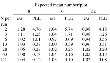
(ii) Accuracy and precision of density estimates The averages of 10 runs of 2 to 141 FA plots (i.e., total sample sizes 20 to 1410) showed improving precision with increasing numbers of samples and plot size, as expected (Table 1). With two plots per run, PLE's averaged four - six times the estimate for all plot sizes. With up to 19 plots per run, PLE's diminished to±24%± 30%, but the effect of increasing plot size was inconsistent. With larger numbers of plots, however, the gain in precision attributable to sampling on the largest plots was only about half the gain achieved by using equivalent areas of smaller plots. For example, with 19 samples per run, the average PLE on the smallest plots was
± 28%, against± 24% on the largest plots. i.e., with four times the effort, the gain in precision was only± 4%. Similarly, 80 small plots gave a PLE of
± 16%, whereas the same sample area (N = 20) of large plots gave± 24%. This confirms that more precise results are obtained from sampling a larger number of smaller plots than from an equivalent area of larger plots, particularly when sampling
aggregated populations.
Estimates from VA plots paralleled those from the FA plots (Table 2), and for larger samples, restricting the maximum counts of VA plots to 20 plants (1.25 x expected count) gave more accurate estimates than the restriction to 24 plants (1.5 x expected count). (iii) Accuracy and precision of estimates of crown area
Crown area of the population was calculated as 1176 m2/ha (assuming ellipsoidal form). Sampling by
five runs of FA and VA plots which contained expected averages of 16 plants gave unbiased and equally precise estimates over a range of sample sizes
Table 1: Estimated density (e)/actual density (a) from 10 computer sampling runs in a mapped bitterbrush population, using fixed area plots designed to contain averages of 8, 16 and 32 plants per plot. Density (e/a) and sampling error figures (PLE, see text for definition) are relative to the parameter of 1.0. The data used are a sub-set of X- Y co-ordinates of plants mapped by Lyon (1968).
Table 3: Estimated crown area (e)/actual crown area (a) for the five computer sampling runs of fixed area and variable area plots given in Table 2. Density (e/a) and sampling error figures (PLE, see text for definition) are relative to the parameter of 1.0. The data used are a sub-set of X- Y co-ordinates of plants mapped by Lyon (1968).
FA VA
Expected mean number/plot max. no./plot max. no./plot
8 16 32 16/plot 24 20
N per e/a PLE e/a PLE e/a PLE N per e/a PLE e/a PLE e/a PLE
run run
2 1.28 4.76 1.04 5.74 0.98 4.18 2 0.83 3.68 0.99 3.93 0.98 4.15
3 1.11 1.25 1.04 1.71 0.98 1.26 3 0.83 1.36 0.92 1.54 0.83 1.56
6 1.02 1.01 0.97 0.69 0.94 0.56 6 0.81 0.57 1.02 0.64 1.01 0.64
13 1.03 0.37 1.00 0.39 0.96 0.31 13 0.99 0.33 1.04 0.34 1.03 0.35
28 1.05 0.27 1.02 0.25 1.02 0.20 28 1.01 0.23 1.05 0.24 1.04 0.24
63 1.08 0.18 1.04 0.16 1.03 0.13 63 0.99 0.17 1.03 0.17 1.02 0.17
141 1.04 0.12 1.03 0.10 1.02 0.08
Table 2: Estimated density (e)/actual density (a) from five comuter sampling runs in mapped bitterbrush, using fixed area and variable area plots expected to contain
16 plants per plot and maxima of 24 and 20 on any VA plot. Density (e/a) and sampling error figures (PLE, see text for definition) are relative to the parameter of 1. o. The data used are a sub-set of x- Y co-ordinates of plants mapped by Lyon (1968).
FA VA
max. no./plot max. no./plot
16/plot 24 20
N per e/a PLE e/a PLE e/a PLE
run
2 0.76 3.73 0.91 3.95 0.89 4.26
3 0.92 1.50 1.02 1.49 0.99 1.28
6 1.06 0.51 1.15 0.52 1.13 0.54
13 1.02 0.36 1.09 0.37 1.08 0.37
28 1.04 0.22 1.09 0.22 1.08 0.23
63 0.97 0.14 1.03' 0.14 1.01 0.15
from 2 to 63 plots per run (Table 3). Because crown area is the product of density and the crown area of each plant, variance of crown area per hectare was slightly larger than variance for density alone. Whitcombe rata-kamahi forest
(i) Sampling intensity, species recorded, and mean density
The area sampled by V A plots with the target count of 30 stems per tier ranged from 14% - 15% of the corresponding FA sample in the irregular-canopied and possum (Trichosurus vulpecula) -modified associations (1 and 2, Table 4) and 28% - 29% in
the closed-canopied and lower altitude associations (3 and 4, Table 4).
Altogether, 29 species were recorded in the FA plots, and 27 in the V A plots. Pink pine (Dacrydium biforme, 10/ha on FA plots) and inanga
(Dracophyllum longifolium, 5/ha on FA plots) were not recorded on VA plots, probably because of chance associated with the smaller areas sampled.
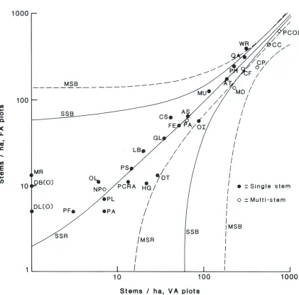
The estimated densities of the taller, single-stemmed species were closely correlated on the two plot-types at the expected ratio of 1: 1 (Fig. 1): Dv A
= 1.04 x DFA -1.009 stems/ha (r2 = 0.954). Only three species, all estimated at less than 10/ha on the FA plots, departed markedly from the regression line - probably also a chance effect of the lower intensity of sampling on the V A plots. In contrast, the V A estimates for the multi-stemmed shrubby species, Coprosma ciliata, C. foetidissima, C. pseudocuneata, weeping matipo (Myrsine divaricata), and pepperwood (Pseudowintera colorata), averaged about 25% more than expected from the FA plots and regressed at greater than the expected 1:1 ratio: DVA = 1.25 x DFA + 12.2 stems/ha (r2 = 0.966). At the association level, this difference amounted to increases of 28% and 23% in associations 1 and 2 (Table 4), where density of the five shrubby species was high (2490 and 3450 stems/ha by FA and V A sampling respectively), but only + 3% and -7% in associations 3 and 4
BATCHELER AND CRAIB: VARIABLE PLOT SAMPLING 87
Figure 1:Log-log plot of stems/ha in the Whitcombe River survey area. Solid diagonal line "SSR"isthe linear regression relationship for single-stemmed species. "MSR"isthe regression for multi-stemmed species. The "MSB" and "SSB" lines are standard error boundaries of the two regressions.
Abbreviations used are:
AT Archeria traversii; AS Aristotelia serrata; CS Carpodetus serratus; CC Coprosma ciliata; CF C. foetidissima; CP C. pseudocuneata; DB Dacrydium biforme*; DL Dracophyllum longifolium"; DT D. traversii; FE Fuchsia excorticata; GL Griselinia littoralis; HG Hoheria glabrata; LB libocedrus bidwillii; MR Melicytus ramiflorus* *; MU Metrosideros umbeIlata; MD Myrsine divaricata; NP Neomyrtus pedunculata; OI Olearia ilicifolia; OL. O. lacunosa; PA Phyllociadus alpinus; PF Podocarpus ferrugineus; PH P. hallii; PA Pseudopanax arboreum; PCRA P. crassifolium; PL P. lineare; PS P. simplex; PCOL Pseudowintera colorata; QA Quintinia acutifolia; WR
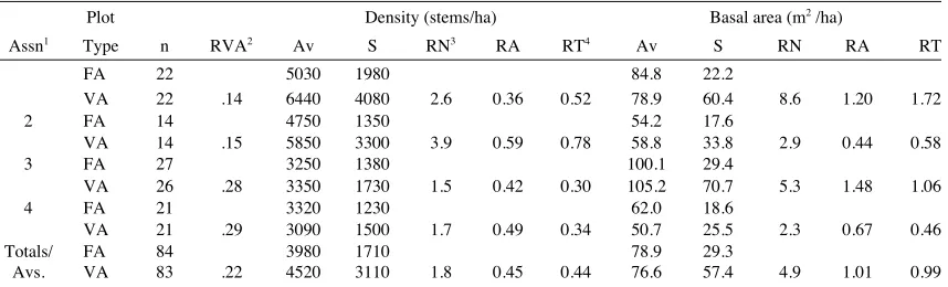
Table 4: Means (Av) and standard deviations (S) of stem densities and basal areas by 20m x 20m fixed area (FA) and variable area (V A) sampling with taret counts of 30 stems per plot in the Whitcombe River survey area, and the estimated V A sampling requirements to obtain precision equal to that obtained by FA sampling.
Plot Density (stems/ha) Basal area (m2 /ha)
Assn1 Type n RVA2 Av S RN3 RA RT4 Av S RN RA RT
FA 22 5030 1980 84.8 22.2
VA 22 .14 6440 4080 2.6 0.36 0.52 78.9 60.4 8.6 1.20 1.72
2 FA 14 4750 1350 54.2 17.6
VA 14 .15 5850 3300 3.9 0.59 0.78 58.8 33.8 2.9 0.44 0.58
3 FA 27 3250 1380 100.1 29.4
VA 26 .28 3350 1730 1.5 0.42 0.30 105.2 70.7 5.3 1.48 1.06
4 FA 21 3320 1230 62.0 18.6
VA 21 .29 3090 1500 1.7 0.49 0.34 50.7 25.5 2.3 0.67 0.46
Totals/ FA 84 3980 1710 78.9 29.3
Avs. VA 83 .22 4520 3110 1.8 0.45 0.44 76.6 57.4 4.9 1.01 0.99
Note 1. Associations with> 5 plots. (1) uneven-canopied Hall's totara and rata with kamahi, Quintinia, cedar, pink pine. (2) Possum-modified cedar, totara, rata, over broadleaf (Griselinia littoralis), ribbonwood (Hoheria glabrata). (3) Closed-canopied rata, kamahi, totara, Quintinia. (4) Lower altitude kamahi, rata, Hall's totara, with occasional miro (Podocarpus ferrugineus) and rimu (Dacrydium cupressinum).
Note 2. R VA is average area of V A plots, relative to the FA plots.
Note 3. RN and RA are estimated numbers and areas of V A plots relative to those of FA plots required to obtain equal precision to that obtained on FA plots.
Note 4. R T is the estimated sampling time for VA plots relative to FA plots, based on the assumed sampling rate of 5 V A plots per 20m x 20m FA plot.
The substantial differences between the two methods for associations 1 and 2 was probably the effect of the different tier height boundaries and measurement protocols when applied to dense populations of thin stems which form a tier at 2-3 m crown height: undoubtedly, many of these were recorded in the> 2 m tier on the VA plots, but not on the FA plots. If this is true, we obviously failed to appreciate the potential importance of the slightly different tier boundary protocols on the FA and V A plots when applied to forests which include a high proportion of shrubs.
(ii) Basal Area
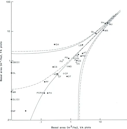
The average basal area of the four associations determined from V A plots was not significantly different from the average on FA plots (Table 4). For species which exceeded about 1 m2 /ha on all plots combined, the averages were closely correlated at the expected 1:1 ratio (Fig. 2). Uncommon or rare species, pink pine, Olearia lacunosa, inanga and mahoe (Melicytus ramiflorus), were either not recorded at all or recorded only rarely on the V A plots. There was no difference between the regressions for single-stemmed and multi-stemmed species (p > 0.01). All 29 species were therefore
pooled to give the linear equation GVA = 1.05 x GFA - 0.1 m'/ha, (r2 = 0.97, G is basal area). i.e. the two methods gave equal estimates of basal areas. Clearly, the high count of small shrubby plants on the VA plots imparted negligible bias to the basal area estimates.
(iii) Precision and sampling requirements
Coefficients of variation expressed as a percentage (CV%) of stem density in the FA plots from the four associations averaged 37%, whereas those for V A plots averaged 48.5%. Corresponding CV%'s of basal areas average 29.5% and 62.9% respectively, so the V A plots were less precise for estimation of both parameters. Using the relationship nVA = nFA. (CVVA/CVFA)2 (where vVA is predicted number of
V A plots, nFA = observed number of FA pots,
BATCHELER AND CRAIB: VARIABLE PLOT SAMPLING 89
as those obtained by FA sampling. For basal area, 101 % of the FA plot area and 99% of the total time are required. That is, in terms of labour
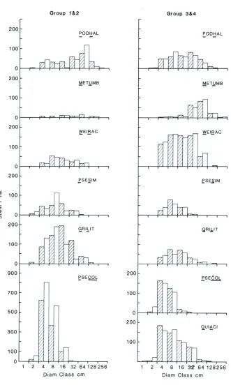
requirements, V A sampling appears to be about twice as efficient for estimating density, and equally efficient for estimating basal area as FA sampling. (iv) Stem diameter frequency distributions. Stem diameters of the common shrubs and trees show good agreement for all species except Hall's totara (Podocarpus hallii) and pepperwood in the irregular-canopied associations (Fig. 3). For Hall's totara, the FA plots yielded a unimodal distribution of size-classes, ranging from the 2 cm lower limit of measurement to a mode between 32-63 cm d.b.h. and occasional trees between 128-256 cm d.b.h.. In contrast, VA sampling portrayed a bimodal distribution, centred on 4-8 cm d.b.h. and 32-64 cm d.b.h.. We don't know which, if either, distribution is true, but it would seem reasonable to expect that the higher intensity of sampling by FA plots would favour the unimodal pattern. For pepperwood, the most abundant species recorded in the irregular-canopied forests, the shapes of the diameter distributions are similar, but the VA estimates are consistently higher than those from FA sampling. This, as noted earlier, is the suspected consequence of the tier boundaries and measurement protocols used in the two methods.
Cupola Basin beech forest
(i) Numbers of species and observations
Although the average numbers of stems (1970) and plants (1981) measured per VA plot ranged widely, the overall averages were close to the intended 30 per plot (Table 5). However, of the 36 woody species in the forest at Cupola Basin (C.M.H. Clarke, unpubl.), only 16 were recorded in both surveys, six in 1970 only, four in 1981 only, and 12 not at all. The most notable unrecorded species were Hall's totara, which occurs sparsely on one hill face of the basin, and cedar (Libocedrus bidwillii), which occurs at low density on swampy moraine over an area of about 20 ha. The other unrecorded species are extremely rare.
Of the 16 species recorded in both surveys, 92% of the total records were for only five: mountain beech, the most abundant, Coprosma pseudocuneata, mountain toatoa (Phyllocladus alpinus), weeping matipo and silver beech (N. menziesii) (Table 5). (ii) Average plant densities
The average density of individual stems obtained from the two surveys was remarkably consistent (20070/ha and 19470/ha for 1970 and 1981 respectively), but it is obvious from the 1981 data that those figures about double the probable average density of 'plants' in the area (Table 5). Nevertheless, there is a close similarity in total stem densities and the relative abundance of species recorded at least 10 times during each survey, despite the 11-year interval between the surveys (r2 = 0.792, P < 0.01).
(iii) Basal Areas
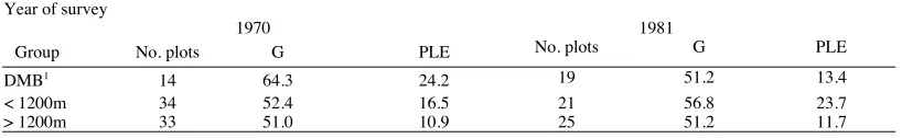
The estimates of basal area in 1970 and 1981 were similar (Table 5). Mountain beech comprised 87% of the total; silver beech and red beech (N. fusca) made up 9%; all other species contributed only 5%. Altogether, the difference between the surveys was 2.8m'/ha, with associated PLE's of :t 16.5% and :t 16.9%, and a maximum difference of 2.3m'/ha for any species. By forest groups, estimates of basal area ranged from 51.0m2/ha to 64.3m2/ha in 1970, and from 51.2m2/ha to 56.8m2/ha in 1981 (Table 6). PLE's, which ranged from ± 21 %-38% in 1970, and from ± 23 % -42 % in 1981, were consistently larger than for all plots combined.
These results indicate that, in beech forests, a change over time of about 16% of basal area could be measured at the 95% confidence level by using 70-80 single-tier V A plots.
Discussion
Accuracy and precision of the method
The computer study of Lyon's bitterbrush confirms the conclusions of other authors (e.g., Bormann, 1953; Kirby, 1965) that in aggregated populations, small plots are more efficient than an equal area of large plots. It also showed that when the computer was constrained "to be a good judge" of the V A required to obtain about the nominated number of plants in each plot (hopefully simulating a human observer in the field), the methods were equally precise. Thus V A sampling passed the first essential test; it yielded accurate and precise estimates of exactly known density and crown area parameters.
Results from the Whitcombe Valley study showed that VA sampling gave similar estimates to those from FA samples for basal area in all four associations sampled, and for total stem density in the two closed-canopied forest associations. But we obviously erred in not anticipating the effect of the slight difference between the FA and VA
BATCHELER AND CRAIB: VARIABLE PLOT SAMPLING 91
Table 5: Numbers of stems and plants counted on V A plots, and estimated densities and basal areas per hectare, from surveys at Cupola Basin in 1970 and 1981.
Stems Plants %1 Numbers/ha Basal area
counted counted both stems stems plants (m2/ha)
Species 1970 1981 1981 years 1970 1981 1981 1970 1981
Mountain beech 1258 1215 1099 44.0 8960 6810 5680 46.3 44.9
Silver beech 185 213 189 7.1 780 930 820 1.9 4.2
Red beech 20 13 13 0.6 70 60 65 2.5 0.6
Mountain toatoa 302 410 153 12.7 3690 2990 940 1.3 0.4
Cop. pse.2 325 793 281 19.9 2810 5430 1740 0.6 0.5
Snow totara 72 49 29 2.1 1270 550 280 0.4 0.1
Weeping maupo 172 302 119 8.4 740 1480 560 0.3 0.2
Dra. uni. 46 23 10 1.2 790 530 200 0.1 0.1
Cop. par. 28 28 28 1.0 240 80 80 0.2 <0.1
Others 72 89 64 2.9 720 610 395 0.3 0.1
Totals 2480 3135 1985 20070 19470 10760 53.9 51.1
Averages/ plot 30.6 44.1 27.9 PLE 8.9 8.6
Ranges No. plots 81 71
lower 9 9 7
upper 56 119 56
Notes: 1. % both years is the total contribution to the stem count for both surveys combined. 2. Abbreviated species names: Cop. pse. Coprosma pseudocuneata, Cop. par. C. parviflora, Dra. uni. Dracophyllum uniflorum. densities of shrubby plants which exceeded 1.35 m
height but were less than 2 cm d.b.h..
Precision of the V A estimates for density accorded with what would be expected from a prediction based on comparison of two sizes of FA plots (Freese, 1961). Using the data in Table 4, the expected average VA CV% for all plots was 54%; the observed average was 55%. Equivalent estimates for expected precision of basal area sampling gave 44.1 %; the observed CV% was 62.9%. i.e., VA sampling for basal area was less precise than expected. Although this confirms that a primary sampling unit chosen for efficiency of estimation of a particular parameter is unlikely to be equally efficient for estimation of other parameters (Wensel and John,
Table 6: Basal areas (G, m/ha) and sampling errors of three groups of forest at Cupola Basin, as determined by single-tier variable area surveys during 1970 and 1981.
1969), V A sampling was about twice as efficient as 20 m x 20 m FA sampling of density, and equally efficient for the estimation of basal area. To achieve this, about four times as many VA plots need to be established.
The two surveys at Cupola Basin gave similar estimates of density and basal area of the total forest and the major species, and indicate that, using temporary plots, 70-80 single-tier plots can detect basal area changes of about ± 16%, or, within the broad forest groups, changes of about 20%-40% with 14-34 plots. Smaller differences would probably be detectable if plots were permanently marked and pairing tests of differences were used.
Year of survey
1970 1981
Group No. plots G PLE No. plots G PLE
DMB1 14 64.3 24.2 19 51.2 13.4
< 1200m 34 52.4 16.5 21 56.8 23.7
> 1200m 33 51.0 10.9 25 51.2 11.7
93 BATCHELER AND CRAIB: VARIABLE PLOT SAMPLING
Having already shown that VA sampling gave unbiased and precise estimates of exactly known parameters (bitterbrush) and of the 'parameters' of the 33,800 m2'universe' of the FA plots
(Whitcombe), it seems reasonable to conclude that the Cupola Basin estimates are also unbiased and reliable. Therefore, we conclude that little, if any, change of basal area or abundance of the common woody plants occurred during the 11-year interval. Although this conclusion suggests that the two similar estimates are evidence that the VA method is repeatable, the argument contains an obvious element of circularity. Nevertheless, C.L.B. spent several hundred days in Cupola Basin during the 1960's and early 1970's and revisited the area in 1981 to look for evidence of the effects of
commercial harvesting of deer(Cervus elaphus)and chamois(Rupicapra rupicapra).Little change was seen in the forest. The canopy had a few new small gaps attributable to storms sometime during the late 1970's. Consistently, the average basal area was about the same (Table 5). The understorey, in which most change was expected, contained only a sprinkling of palatable shrubs which were occasionally seen but rarely occurred on the plots. On balance, we consider that the structure and composition of the forest did not change in any significant way and therefore, that the conclusion on repeatability is valid.
The general conclusion therefore is that V A sampling of the kind described is a particularly flexible form of polyareal sampling (Husch, Miller and Beers, 1972) in which probability of selection is entirely proportional to frequency (Grosenbaugh and Stover, 1957). Variations of numbers of plants recorded on individual plots therefore appears to be a "random noise" effect which may affect precision, but does not appear to bias the estimates.
Application to surveys
Regardless of the sampling method, interpretation of a forest inventory is inevitably based on a condition concept such as that outlined in the Introduction, autecological knowledge of the plants, and synecological knowledge of the "normal" forest.
Studies by Wardle (1970, 1984), Franklin (1965), Mark et al (1964), Mark (1963), Scott, Mark and Sanderson (1964), Mark and Sanderson (1962) and the results from Cupola Basin indicate that average basal areas of beech forests increase with altitude and rainfall from about 40 m2/ ha to more than 100
m'/ha, with extreme values in "climax" stands in the
order of 200 m2/ha. Westland rata - kamahi forests
range up to about 150 m2/ha. At Haupiri, North
Westland, the average, including tree ferns, was 112 m2/ha (Coleman, Gillman and Green, 1980).In
the Taipo River valley, it was 104 m2/ha, excluding
tree ferns, and approximately 125 m2/ha including
tree ferns (D.G.C. unpubl. data). Further west, in lower rainfall, forests in the Whitcombe River Valley averaged 87 m2/ha in 1971 (I. L. James, unpubl.
data) and 77-79 m2/ha in 1982-83 (Table 4).
By way of contrast, in the Kokatahi Valley, a tributary of the Hokitika River, basal area averaged 27 m2/ha two decades after possums had reached
high numbers (I. L. James, unpubl. data). Compared with adjacent forests, this indicates the loss of about 70% of the biomass of the Kokatahi forest. Similarly, our results from the Whitcombe gave 54-59 m2/ha (FA and V A sampling respectively) for
the association which appeared to be most damaged by possums. Compared with an average of 87 m2
obtained a decade earlier by James (unpubl.), possum browsing appears to have reduced basal area of the living forest by about one-third.
Thus basal area can be, as suggested in the Introduction, an illuminating measure of the over-all change, at least where animal (possum) damage is concentrated on the larger trees. But we recognise that much more information is necessary before patterns and norms can be developed for the indigenous forests which are sensitive to canopy damage.
amount of field work, the V A method was about twice as precise for estimating density as were 20 m x 20 m FA plots. Furthermore, as was found in all three field studies reported, the total numbers of stems or plants included in the inventories was very close to the target counts so, in general, the total data-base from a V A survey is quite predictable. Thus on the grounds of accuracy, precision, predictability of the data base, and relative efficiency of larger numbers of small samples for estimation of aggregated populations, V A methods appear to be particularly suitable for large-scale surveys of New Zealand's indigenous forests.
Acknowledgements
We acknowledge the generosity of L Jack Lyon for permitting the use of his bitterbrush data and the help given by many colleagues and vacation works in the field and statistical laboratory, particularly Jill Andrews, Dorothy Batcheler, I. L James, M. J. McLennan, G. T. Jane, K. H. Platt and C. M. H. Clarke. We also gratefully acknowledge the critiques of earlier drafts of this paper by
E. B. Spurr, J. Orwin, M. J. McLennan and the Hon. Editor.
References
Allen, R. B.; McLennan, M. J. 1983. Indigenous forest survey manual: two inventory methods.
Forest Research Institute Bulletin48: 73 pp. Allen, R. B.; Payton, I. J.; Knowlton,J. E. 1984.
Effects of ungulates on structure and species composition in the Urewera forests as shown by exclosures.New Zealand Journal of Ecology7: 119-30.
Batcheler, C. L; Wardle, J. A. 1977. Vegetation and animal condition assessments in National Parks. In:Seminar on science in national parks1976. pp 109-21. New Zealand National Parks Authority, Wellington 373 pp.
Bormann, F. H. 1953. The statistical efficiency of sample plot size and shape in forest ecology.
Ecology34: 474-87.
Coleman, J. D.; Gillman, A.; Green, W. Q. 1980. Forest patterns and possum densities within podocarp/mixed hardwood forests on Mt Bryan O'Lynn, Westland.New Zealand Journal of Ecology3: 69-84.
Eberhardt, L L 1967. Some developments in "distance sampling".Biometrics23: 207-16. Franklin, D. A. 1965. Quantitative data on forest
composition.New Zealand Journal of Botany3 : 168.
Freese, F. 1961. Relation of plot size to variability: an approximation.Journal of Forestry59: 679. Greig-Smith, P. 1957.Quantitative plant ecology.
Butterworths, London, 198 pp.
Grosenbaugh, L R.; Stover, W. S. 1957. Point sampling compared with plot sampling in southeast Texas.Forest Science3: 2-14. Holloway, J. T.; Wendelken, W. J. 1957. Some
unusual problems in sample plot design.New Zealand Journal of Forestry7(4): 77-83. Husch, B.;Miller, K. I.; Beers, T. W. 1972.Forest
mensuration.Ronald, N.Y. 490pp. Jane, G. T. 1982. Constant count - a solution to
problems of quadrat size.New Zealand Journal of Ecology5: 151-2.
Kirby, C. L 1965. Accuracy of point sampling in white spruce - aspen stands of Saskatchewan.
Journal of Forestry63: 924-26.
Lyon, L J. 1968. An evaluation of density sampling methods in a shrub community.Journal of Range Management21: 16-20.
Mark, A. F. 1963. Vegetation studies on Secretary Island, Fiordland. Part 3. The altitudinal gradient in forest composition, structure and regeneration.New Zealand Journal of Botany1: 188-202.
Mark. A. F.; Sanderson, F. R. 1962. The altitudinal gradient in forest composition, structure and regeneration in the Hollyford Valley, Fiordland.
Proceedings of the New Zealand Ecological Society9: 17-26.
Mark, A. F.; Scott, G. A.M.;Sanderson, F. R.; James, P. W. 1964. Forest succession on landslides above Lake Thomson, Fiordland.
New Zealand Journal of Botany2: 60-89. Mark, A. F.; Scott, G. A. M. 1965. Notes and
comments.New Zealand Journal of Botany3: 168-69.
Scott, G. A.M.;Mark, A. F.; Sanderson, F. R. 1964. Altitudinal variation in forest composition near Lake Hankinson, Fiordland.New Zealand Journal of Botany2: 310-23.
Stewart, G. H.; Veblen, T. T. 1982. Regeneration patterns in southern rata(Metrosideros umbellata)- kamahi(Weinmannia racemosa)
forest in central Westland, New Zealand.New Zealand Journal of Botany20: 55-72. Wardle, J. A. 1970. The ecology ofNothofagus
BATCHELER AND CRAIB: VARIABLE PLOT SAMPLING 95
Wardle, J. A. 1984. The New Zealand beeches. Ecology, utilization and management. New Zealand Forest Service. 447 pp.