A Novel Approach Canberra Measure Minimal Spanning Tree Using Fuzzy C-Means Based on Gaussian Function for Image Data Mining

http://www.sciencepublishinggroup.com/j/acis doi: 10.11648/j.acis.20180605.11

ISSN: 2328-5583 (Print); ISSN: 2328-5591 (Online)

A Novel Approach Canberra Measure Minimal Spanning

Tree Using Fuzzy C-Means Based on Gaussian Function for

Image Data Mining

Senthil

1, *

, Nithya

2

, Bhuvaneswari

2

1_{Department of Economics and Statistics, Government of Tamilnadu, DRDA, Dindigul, India} 2

Department of Mathematics, Mother Teresa Women’s University, Kodaikanal, India

Email address:

*

Corresponding author

To cite this article:

Senthil, Nithya, Bhuvaneswari. A Novel Approach Canberra Measure Minimal Spanning Tree Using Fuzzy C-Means Based on Gaussian Function for Image Data Mining. Automation, Control and Intelligent Systems. Vol. 6, No. 5, 2018, pp. 54-61.

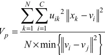
doi: 10.11648/j.acis.20180605.11

Received: February 13, 2019; Accepted: March 14, 2019; Published: April 3, 2019

Abstract:

Clustering analysis has been an emerging research issue in data mining due to its variety of applications. In recently, mathematical algorithm supported automatic segmentation system plays an important role in clustering of images. The fuzzy c-means clustering is a method of cluster analysis which aims to partition n data points into k-clusters. The conventional FCM-based algorithm considers no spatial content information, which means it sensitive to noise. Unsupervised techniques need to be employed, which can be based on minimal spanning tree generated by comparing spatial neighbourhood information, the MST based clustering algorithms have been widely used due to their ability to detect clusters with irregular boundaries. We propose an automatic fuzzy c-means initialization algorithm based on Canberra distance minimal spanning tree for the purpose of segmentation of medical images, where vertices and edges are labelled with multi-dimensional vectors. A Canberra distance measure based, construct the minimal spanning tree clustering algorithm. An efficient method for calculating membership and updating prototypes by minimizing the new objective function of Gaussian based fuzzy c-means. The algorithm uses a new cluster validation criterion based on the geometric property of data partition of the dataset in order to find the proper number of cluster at each level. In this algorithm to apply medical images to reduce the inhomogeneity and allow the labelling of a pixel to be influenced by the labels in its immediate neighbourhood and reduces the time complexity and better clustering results than the existing traditional minimal spanning tree algorithm. The performance of proposed algorithm has been shown with random data set, partition coefficient and validation function are used to evaluate the validity of clustering and then new cluster separation approach to optimal number of clustering. Also this paper compares the results of proposed method with the results of existing basic fuzzy c-means.

Keywords:

Fuzzy C-Means, Gaussian Function, Lagrange Multiplier, Canberra Distance, Minimal Spanning Tree, Cluster Separation, Partition Coefficient, Validation Function

1. Introduction

Clustering is one of the important tools for data analysis. It can divide an unlabeled dataset into several subsets according to some criteria to ensure similar samples to be in the same subset and dissimilar samples to be different subset. Fuzzy c-means algorithm is a widely used clustering algorithm in the field of machine learning. It was proposed by Bezdek et al in 1984 [1]. By introducing the fuzzy membership matrix, the

patients body and patients motion. So the medical MRI is seriously affected and it has improper information about the anatomic structure. Hence the segmentation of medical images is an important one before it to go for treatment planning for proper diagnosis. Initially segmentation was made manually; but manual segmentation is more difficult, time -consuming and costly. Automatic brain tumor segmentation from MR images which is not an easy task that involves various disciplines covering image analysis, mathematical algorithms [8-10] and etc.

In recent world, many of the segmentation methods are based on the unsupervised clustering algorithms. Unsupervised clustering is a process for ordering objects in such a way that samples of the identical group are more similar to one another than samples belonging to different groups. Currently fuzzy c-means of fuzzy clustering plays main role in unsupervised clustering method for segmenting medical images [11]. In Noordam, proposed a geometrically guided FCM algorithm based on a semi-supervised FCM technique for multivariate image segmentation. In their work, the geometrical condition information of each pixel is determined by taking into account the local neighbourhood of each pixel [5].

The main disadvantages of fuzzy clustering technique are its need for a large amount of time to converge and it is more sensitive to the noise and outliers in the data, because of squared-norm to measure similarity between prototypes and data points. To cluster more general dataset, lots of algorithms have been proposed by replacing the squared-norm with other similarity measures. A recent development is to use kernel method to construct the kernel versions of FCM algorithm, KFCM for clustering the incomplete data and medical image segmentation was proposed [12-13]. However a disadvantage of KFCM in segmentation of medical images it is not considered about any spatial information in image context; which makes it compute the neighbourhood term in each step, which is very time consuming. Although the above methods are claimed to be robust to noise, they are confronted with the problem of selecting the parameters that control the role of the spatial constraints. However, FCM has two serious shortcomings, Firstly, it easily falls into local minima, Secondly, it is necessary to specify the number of clusters and the algorithm is very sensitive to the initial center [14-15]. The graph data structure is being considered as a suitable mathematical tool to model the inherent relationship among data. Simple linked data are generally modeled using simple graphG=( , )V E , where V is the set of vertices representing key concepts or entities and E⊆ ×V V

is the set of links between the vertices representing the relationships between the concepts or entities. There are many complex data link online social networks, where is characterized by a set of features and multiple relationships exist between an entity pair, such data, the concept of graph can be used where in each vertex is represented by an n-dimensional vector. One of the important tasks related to graph data analysis is to decompose a given graph into multiple cohesive subgraphs, called clusters, based on some

common properties. The clustering is an unsupervised learn process to identify the underlying structure of data, which is generally based on some similarity/ distance measures between data elements.

Graph clustering is special case of clustering process which divides an input graph into a number of connected components such that intra-component edges are maximum and inter- components edges are minimum. Each connected components is called a cluster [16]. Graph clustering techniques on the minimum spanning tree (MST) of a weighted graph is minimum weight spanning tree of that graph with the classical MST algorithms [17, 18, 19] and the cost of constructing a minimal spanning tree is O m( log )n , where m is the number of edges in the graph and n is the number of vertices. Our study on these methods have led us to believe that all these applications have used the MSTs in some heuristic way; eg cutting long edges to separate clusters without fully exploring their power and understanding their rich properties related to clustering. Geometric notion of centrality are closely linked to facility location problem. Since similarity/ distance measure is the key requirement for any clustering algorithm, In this paper, we have proposed a new weighted distance measure based on weighted Euclidean norm to calculate the distance between the vertices and the algorithm is initialized by a given kernel function using minimal spanning tree based FCM algorithm, which helps to speed up the convergence of the algorithm.

The rest of the paper is organized as follows section 2 presents a Canberra distance measures and Cluster Separation using CMST clustering algorithm. Section 3 presents the kernel based FCM and Validation function. Section 4 presents the experimental results using random data show that the proposed method can achieve comparable results to those from many derivatives of efficient initialized by a given kernel function using minimal spanning tree based FCM algorithm and effective and more robust to reduce the noise and outliers.

2. Canberra Measure Based minimal

Spanning Tree Algorithm

In this section, we proposed Canberra distance measures for construct the minimal spanning tree.

2.1. Canberra Distance Measure MST

Given the grayscale point set D, the hierarchical methods starts by constructing a minimal spanning tree (MST) from the points in D. In x=( ,x x_{1 2},...x_n)T and

1 2

( , ,... _n)T

y= y y y are two points of a MST and e x y( , )is an edge between x and y then the Canberra distance between x and y is denoted by d x y( , )and calculated using equation (1) [20],

1

1 ( , )

n

i i

i i

i

x y

d x y _K

x y

= − =

+

∑

(1)

2.2. Cluster Separation (CS)

The definition of CS between cluster centers is given by the following

min

max

E CS

E

= (2)

where E_maxis the maximum length edge in the MST, which represents two centroids that are at maximum separation and

min

E is the length edge in the MST, which represents two centroids that are nearest to each other. Then the CS represents the relative separation of the centroids. The value of CS ranges from 0 to 1. A low value of CS means that the two centroids are too close to each other and the corresponding MST Separation not valid. A high CS value means the MST separation of the data is even and valid. If the CS is greater than the threshold, the MST partition of the dataset is valid. Then, we increase the number of cluster by and test the CS again. This process continuous until the CS is smaller than the threshold. The value setting of the threshold for the CS will be practical and is dependent on the dataset. The higher the value of the threshold the smaller the number of clusters would be, generally the value of the threshold will be ≻0.8[21].

2.3. Canberra Distance Based Minimal Spanning Tree Algorithm

Algorithm: CMST Input: Data points

Output: optimal number of cluster centers

Let e1 be an edge in the CMST1 constructed from data points Let e2 be an edge in the CMST2 constructed from C. Let S_Tbe the set of disjoint subtrees of CMST1. 1. Create a node v, for each data points. 2. Compute the edge weight using equation (1) 3. Construct an CMST1 from 2

4. S_T =

ϕ

, n_c=1 ,C=

ϕ

. 5. Repeat.

6. For eache1∈CMST1.

7. Current longest edge e remove e1 from CMST1. 8. S_T =S_T ∪{ }/ /T' T'is new disjoint subtrees (regions). 9. n_c= +n_c 1.

10. Compute the center c of T_{i i}using average of points.

11. { }

i

T T i

C=∪ ∈S c .

12. Compute the edge weight using equation (1) 13. Construct an CMST2 T from C.

14. E_min=get-min length edge. 15. E_max=get-max length edge.

16. min

max

E CS

E

=

17. Until CS<0.8

18. Merge the closest neighbour from CMST2.

19. Update the clusters points, repeat step 12 to step 18. 20. Finally we obtain the cluster centers.

3. Formulation of Proposed Kernel

Function Induced FCM Based on

Gaussian Function

3.1. Fuzzy C-Means Algorithm

This method was first introduced by Dunn in [22] and improved by Bezdek in [23]. It is based on minimization of the following objective function:

2

1 1

( , )

N C

m

m ij i j

i j

J U V u x c

− =

=

∑ ∑

− 1< < ∞m (3)

where m is any real number greater than 1, uij is the degree of membership of xi in the cluster j, xiis the i

th

of p - dimensional measured data, cj is the p -dimension center of the cluster and ∗ is any norm expressing the similarity between any measured data and center.

Fuzzy partitioning is carried out through an iterative optimization of the objective function shown above, with the update of membership uij and the cluster centers cj by:

2 1

1

1

ij

c m

i j

i k

k

u

x

c

x

c

−

=

=



₋







−









∑

(4)

1

1

N m ij i i

j _N

m ij i

u x

c

u

=

= =

∑

∑

(5)

This iteration will stop when

{

1

}

maxij uijk+ −uijk <∈,

where ∈ is a termination criterion between 0 and 1, whereas k is the iteration steps. This procedure converges to a local minimum or a saddle point of J_m.

3.2. Kernel Function Induced FCM Algorithm

Recently, the powerful technique of kernel function using learning machines were proposed and found to have successful applications such as signal processing pattern recognition and image processing etc. Kernel method often studies and employs a high-dimensional feature space S for having nonlinear classification boundaries. For this a mapping is given below;

: Rp S

ϕ

→ is used where by an object x is mapped into S:

1 2

( )

x

(

( ),

x

( ),...)

x

As x is the p-dimensional vector,

ϕ

( )x may have the infinite dimension. In the nonlinear classification method, an explicit form of

ϕ

( )x is unavailable, but the inner product is defined by:

( , ) ( ), ( )

K x y =

ϕ

x

ϕ

y

The function K x y( , )is called a kernel function and we assume this known function, as Gaussian radial basis function: 2 2 2 ( , ) x y

K x y e σ

− − =

This paper proposes an efficient weighted MST based FCM by introducing kernel function that allows the clustering of objects to be more reasonable. The modified proposed objective function is given by

2

1 1

( , ) ( ) ( )

N C

m

m ik k i

k i

J U V u

ϕ

x

ϕ

v

= =

=

∑ ∑

− (6)

where ϕ stands as map and the distance function can be expressed using in product space as

2

( ) ( ) ( ), ( ) ( ), ( )

2 ( ), ( )

k i k k i i

k i

x v x x v v

x v

ϕ

ϕ

ϕ

ϕ

ϕ

ϕ

ϕ

ϕ

− = +

−

To obtain kernel induced FCM based Gaussian function the distance function can be modified as

2

(x_k) ( )v_i G x x( _k, _k) G v v( , ) 2 (_{i i} G x v_k, )_i

ϕ

−

ϕ

= + − where

1, 2, 3...

k= N andi=1, 2, 3...C.

Let us expressG x v( _k, )_i , between pixel x_k and v_i as the product of a feature similarity term and spatial proximity term:

2 2

2 2

( ) ( )

( , ) exp exp

2 2

k i k i

k i

X I

x v I x I v

G x v

σ σ _{− −}  _{− −}      = ∗         (7)

where σ is a parameter which can be adjusted by users. Using the above expression, we obtain G x x( _k, _k) 1= and

( , ) 1_{i i}

G v v = , so the distance function can be rewritten as

2

(x_k) ( )v_i 2 (1 G x v( _k, ))_i

ϕ

−

ϕ

= − (8)

Substituting kernel induced Gaussian function based FCM is given by

1 1

( , ) 2 (1 ( , ) )

N C

m

m ik k i

k i

J U V u G x v

= =

=

∑ ∑

− (9)

3.3. Obtaining Membership

To obtain equation for calculating membership we minimizing the objective function

1 1

( , ) 2 (1 ( , ) )

N C

m

m ik k i

k i

J U V u G x v

= =

=

∑ ∑

− (10)

subject to the constraints

1 1 C ik i u = =

∑

Therefore, the above objective function can be minimized using one Lagrangian multiplier:

1 1 1

( , , ) 2 (1 ( , ) )) 1

N C C

m

m ik k i ik

k i i

J U V λ u G x v λ u

= = =

 

= − −  − 

 

 

∑ ∑

∑

(11)

where λ is a Lagrange multiplier.

To adjust u_ik&v_ifor minimum Jm, we set to zero the derivative of J_m( , , )U V

λ

with respect tou_ik for m≻1.

[

]

1

2 m 1 ( 0

m

ik k i

ik J

mu G x v

u λ − ∂ _{= − − − =} ∂

(

)

1 1

1 _{1 ( , )} 1

m m

ik k i

m

u _=λ − G x v −

   

−

To calculateλ , Substitute the above uikin the identity constraint for all values of k, we get following relation,

1

2 ( ) 0

N m m

ik k i

i _k

J

u x v

v ₌

∂ _{= − − =}

∂

∑

The minimum of J_m with respect to v_iwas computed by taking the partial derivative of J_m equal to zero.

1 1 1 1 1 1 1

(1 ( , ))

m C m k i i m

G x v

λ ₋ − =   =        ₋   

∑

So that v_i and u_ikcan be calculated by the relation, we obtain

1 1 1

1

1 ( , )

1 ( , )

ik _C

k i m k j j

u

G x v G x v

− = =  ₋    −    

∑

(12) 1 1 ( ) ( , ) . ( ) ( , ) N m

ik k i k

k

i N

m

ik k i

k

u G x v x

v

u G x v

=

= =

∑

∑

(13)

The kernel function based FCM algorithm iteratively optimizes J_m by continuous updating u_ik and v_iuntil the difference in successive u_ikvalues is very small ≤ ∈, where

4. Efficient Kernel Induced FCM Based

on Gaussian Function

The objective function (I) of the standard FCM algorithm does not take into account any spatial information, which means the clustering process is related to gray levels independently of the pixels of image segmentation. Therefore, the limitation makes FCM to be very sensitive to noise. The general principle of the technique presented in this paper is to incorporate the neighbourhood information into the FCM algorithm during classification.

4.1. Efficient KFCM Algorithm

Stage 1: Set the cluster centroids

{ }

v_{i i}c₌₁ by using Canberra MST initialization method.

Stage 2: Compute the membership function using (12) Stage 3: Update the cluster centroids using (13) Stage 4: Estimate objective function using (10)

Stage 5: Go to stage (2)-(3), repeat until convergence. The termination criterion is as follows J_m−J_m−1 ≺∈ , where m is the iteration count, ∈ is a small number that can be set by the user.

4.2. Validation Function Based on Feature Structures

Two representative functions for the fuzzy partition namely; Partition coefficient V_pc and Validation function V_p

are used to evaluate the validity of clustering [3, 24].

2

1 1

1 N C

pc ik

k i

V u

N _{= =}

=

∑∑

(14)

{

}

2 2

1 1

2

min N C

ik k i

k i p

i j

u x v

V

N v v

= =

− =

× −

∑∑

(15)

The proposed efficient weighted MST obtained cluster centers; the EKFCM algorithm continues iteratively updates, membership and centroids with these values. When this improved, Efficient KFCM algorithm has converged, another defuzzification process takes place in order to convert the fuzzy partition matrix to a crisp partition matrix that is segmented.

5. Results and Discussion

This section describes some experimental results on random data, corrupted with noise to show the segmentation performance of the proposed method.

Table 1. Random data.

Data Data

S. No X Y Intensity S. No X Y Intensity

1 1.80 2.00 0.50 11 12.00 4.00 0.80 2 2.00 2.20 0.91 12 11.50 3.50 0.45 3 2.00 1.80 0.12 13 12.50 3.50 0.55 4 2.00 3.50 0.40 14 21.00 10.00 0.65 5 8.80 3.00 0.50 15 21.00 11.00 0.25 6 9.00 3.20 0.38 16 20.50 10.50 0.35 7 9.00 2.80 0.60 17 21.50 10.50 0.75 8 9.20 3.00 0.12 18 2.00 4.00 0.70 9 7.00 2.80 0.80 19 19.00 20.00 0.60 10 12.00 3.00 0.90 20 11.00 12.00 0.40

Table 2. Dissimilarity matrix-I.

Co-ordinate intensity

S. No x y I(v) S. No 1 2 3 4 5 6 7 8 9 10 11

1 1.8 2.0 0.50 1 0.000 0.130 0.239 0.145 0.287 0.345 0.308 0.495 0.329 0.408 0.434 2 2.0 2.2 0.91 2 0.000 0.289 0.206 0.358 0.411 0.321 0.521 0.247 0.291 0.356 3 2.0 1.8 0.12 3 0.000 0.286 0.498 0.479 0.507 0.298 0.504 0.576 0.611 4 2.0 3.5 0.40 4 0.000 0.273 0.236 0.316 0.419 0.333 0.392 0.371 5 8.8 3.0 0.50 5 0.000 0.060 0.046 0.212 0.126 0.147 0.176 6 9.0 3.2 0.38 6 0.000 0.097 0.188 0.183 0.194 0.203 7 9.0 2.8 0.60 7 0.000 0.237 0.089 0.126 0.154 8 9.2 3.0 0.12 8 0.000 0.303 0.299 0.338 9 7.0 2.8 0.80 9 0.000 0.119 0.147 10 12.0 3.0 0.90 10 0.000 0.067 11 12.0 4.0 0.80 11 0.000 12 11.5 3.5 0.45 12

13 12.5 3.5 0.55 13 14 21.0 10.0 0.65 14 15 21.0 11.0 0.25 15 16 20.5 10.5 0.35 16 17 21.5 10.5 0.75 17 18 2.0 4.0 0.70 18 19 19.0 20.0 0.60 19 20 11.0 12.0 0.40 20

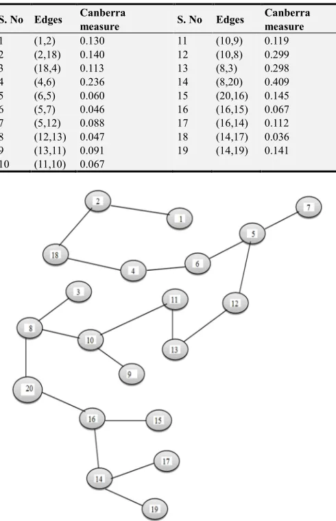
Figure 1 shows a typical example of CMST1 constructed from point set (from Dissimilarity matrix), in which

clusters, which will be useful in many applications.

Table 3. Canberra distance based minimal spanning tree edges.

S. No Edges Canberra

measure S. No Edges

Canberra measure

1 (1,2) 0.130 11 (10,9) 0.119 2 (2,18) 0.140 12 (10,8) 0.299 3 (18,4) 0.113 13 (8,3) 0.298 4 (4,6) 0.236 14 (8,20) 0.409 5 (6,5) 0.060 15 (20,16) 0.145 6 (5,7) 0.046 16 (16,15) 0.067 7 (5,12) 0.088 17 (16,14) 0.112 8 (12,13) 0.047 18 (14,17) 0.036 9 (13,11) 0.091 19 (14,19) 0.141 10 (11,10) 0.067

Figure 1. Canberra distance based Minimal spanning tree connected through points.

Generally in most of the clustering algorithm data points can be represented as dissimilarity matrix representation. It contains the distance values between the data points represented as lower or upper triangular matrix. Our Canberra distance based minimal spanning tree algorithm constructs CMST1 from the dissimilarity matrix is shown figure 1. First to identify the longest edge in the CMST1 to generate subtree (clusters). Table 3, the longest edge weight 0.409 connecting the data points 8 and 20 is find to be inconsistent one. By removing the inconsistent edge from the CMST1, data points in the CMST1 partitioned into two

subtrees or clusters T1 and T2 namely

{

}

1 1, 2, 3, 4, 5, 6, 7,8, 9,10,11,12,13,18

T = and

{

}

2 14,15,16,17,19, 20

T = . Secondly to find the center of T₁

and T₂ using average of points, these centers is connected and again another minimal spanning tree CMST2 is constructed. The minimum edge of CMST2 is Emin =0.750

and the maximum edge of CMST2 is E_max =0.750then to

compute cluster separation value is 1. If the CS is greater than 0.8 then we conclude the subtrees or clusters created are well separated. Next to identify another longest edge weight from Table 3 is 0.299 connecting the data points 10 and 8 is finding to be inconsistent one. By removing the inconsistent edge from the CMST1, data points partitioned into three sub trees or clusters T₁ , T₂ and T₃ namely

{

}

1 1, 2, 4,5, 6, 7,9,10,11,12,13,18

T = ,T₂=

{

14,15,16,17,19, 20

}

and T₃=

{ }

3,8 . To compute the center of T₁,T₂ and T₃

using average of points, these centers is connected and again another minimal spanning tree CMST2 is constructed.

Table 4. Dissimilarity matrix-II.

Cluster-I Cluster-II Cluster-III

Cluster-I 0.000 0.381 0.317 Cluster-II 0.000 0.611 Cluster-III 0.000

Table 5. Canberra distance based CMST2 edges.

S. No Edges Canberra measure

1 (1,3) 0.317 2 (1,2) 0.381

The minimum edge of CMST2 is E_min =0.317and the maximum edge of WMST2 is Emax=0.381then to compute

cluster separation value is 0.832. If the CS is greater than 0.8 then we conclude the subtrees or clusters created are valid. Continuing this process, next to identify another longest edge weight from Table 3 is 0.298 connecting the data points 3 and 8 is finding to be inconsistent one. By removing the inconsistent edge from the CMST1, data points partitioned into three sub trees or clustersT₁,T₂ ,T₃and T₄ namely

{

}

1 1, 2, 4, 5, 6, 7, 9,10,11,12,13,18

T = , T₃ =

{ }

3 and

{ }

4 8

T = . To compute the center of T1,T2,T3 and T4using

average of points, these centers is connected and again another minimal spanning tree CMST2 is constructed.

Table 6. Dissimilarity matrix-III.

Cluster-I Cluster-II Cluster-III Cluster-IV

Cluster-I 0.000 0.381 0.508 0.267 Cluster-II 0.000 0.723 0.523 Cluster-III 0.000 0.298 Cluster-IV 0.000

Table 7. Canberra distance based CMST2 edges.

S. No Edges Canberra measure

1 (1,4) 0.267 2 (4,3) 0.298 3 (4,2) 0.523

The minimum edge of CMST2 is E_min =0.267and the maximum edge of CMST2 is Emax=0.523then to compute

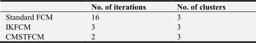
for the given data points. Then the center of the cluster and its convergence of standard FCM and EKFCM are determined under successive interactions of experiments using data points. The standard FCM algorithm and the numbers of updated centers are high under the objective function of Euclidean distance measures. This takes more iteration to converge the termination value of algorithm. With the new efficient objective function based kernel distance measure the termination value is achieved, with very less iteration and with much better performance in getting membership (Table 8) than standard FCM. Table 9 gives the number of iteration to achieve the results of cluster on the data points by standard FCM and EKFCM. It is clear from the final cluster, membership (Table 8), scatter diagram (Fig

2), that our proposed EKFCM is much faster than the standard FCM and the method is converged fast to terminate condition with less run time. To test the effectiveness of EKFCM, the weighted minimal spanning tree based FCM is used as center. This is done to find out the fuzzy membership and appropriate number of clusters. Thus, we have concluded the final optimal clusters formed as 3. This algorithm has also reduced the number of iterations. Best result is achieved by this measure fuzzy partition coefficient V_pc maximum and validation function V_p minimum (Table 10). The EKFCM clustering algorithm has the following membership value intimacy (Table 8).

Table 8. Final membership of three clusters of EKFCM method and object allocation.

Co-ordinate(x, y) intensity

appropriate cluster

S. No x y I(v) Mem-1 Mem-2 Mem-3

1 1.80 2.00 0.50 0.8542 0.0026 0.1432 1 2 2.00 2.20 0.91 0.9940 0.0022 0.0038 1 3 2.00 1.80 0.12 0.0094 0.0002 0.9905 3 4 2.00 3.50 0.40 0.5591 0.0057 0.4352 1 5 8.80 3.00 0.50 0.9462 0.0092 0.0446 1 6 9.00 3.20 0.38 0.5872 0.0259 0.3869 1 7 9.00 2.80 0.60 0.9955 0.0015 0.0030 1 8 9.20 3.00 0.12 0.0131 0.0021 0.9848 3 9 7.00 2.80 0.80 0.9912 0.0050 0.0037 1 10 12.00 3.00 0.90 0.9660 0.0316 0.0024 1 11 12.00 4.00 0.80 0.9545 0.0412 0.0043 1 12 11.50 3.50 0.45 0.8067 0.0536 0.1397 1 13 12.50 3.50 0.55 0.9191 0.0457 0.0352 1 14 21.00 10.00 0.65 0.0255 0.9738 0.0007 2 15 21.00 11.00 0.25 0.0100 0.9753 0.0147 2 16 20.50 10.50 0.35 0.0097 0.9849 0.0053 2 17 21.50 10.50 0.75 0.0382 0.9614 0.0004 2 18 2.00 4.00 0.70 0.9826 0.0035 0.0139 1 19 19.00 20.00 0.60 0.0016 0.9983 0.0001 2 20 11.00 12.00 0.40 0.1090 0.8430 0.0480 2

Figure 2. Scatter diagram for CMST based FCM, final cluster three.

Table 9. Comparison of iteration count.

No. of iterations No. of clusters

Standard FCM 16 3 IKFCM 3 3 CMSTFCM 2 3

Table 10. Cluster validity function.

pc

V V_p

Standard FCM 0.8372 0.2532 IKFCM 0.8423 0.2623 CMSTFCM 0.8705 0.1253

6. Conclusion

pixels and also compares the results with standard FCM segmentation. It is clear from our comparison that EKFCM performed better than FCM. The results accuracy and validation functions used in measuring the efficiency in clustering algorithm with Gaussian. In future we will explore and test our proposed algorithm in various domains.

Acknowledgements

We would like to thank the reviewers for their constructive comments. We thank to Dr. R. David chandrakumar, Professor, Department of Mathematics, Vickram College of Engineering for his encouragement and support given.

References

[1] Bezdek. J. C, Ehrlich. R and Full. W, FCM: the fuzzy c-means clustering algorithm, Computers & Geosciences, Vol. 10, No. 2-3, pp. 191-203(1984).

[2] Mac Queen. J, Some methods for classification and analysis of multivariate observations, In Proceedings of the 5th Berkeley symposium on mathematical statistics and probability, University of California press, USA, pp. 14(1967).

[3] Bezdek J. C., Hall L. O., Clarke L. P, Review of MR image segmentation techniques using pattern recognition, medical physics 20(4), pp. 1033-1048(1993).

[4] Ferahta N., Moussaoui A., Benmahammed K., Chen V, New fuzzy clustering algorithm applied to RMN image segmentation, international journal of soft computing 1(2), pp. 137-142 (2006).

[5] Noordam J. C., Van Den Broek W. H. A. M., Buydens L. M. C, Geometrically guided fuzzy C-means clustering for multivariate image segmentation, In. proceedings15-th International conference on pattern recognition, Vol. pp. 462-465(2000).

[6] Mahipal singh choudhry and Rajiv Kapoor, A novel fuzzy energy based level set method for medical image segmentation, Cogent engineering, vol. 5(2018).

[7] Perumal K and Latha C, Probability based fuzzy c-means for image segmentation, International Journal of Pure and Applied Mathematics, vol. 18 (17), pp. 779-789(2018).

[8] Hall L. O., Bensaid A. m., Clarke L. P., Velthuizen R. P., Silbiger M. S., Bezdek J. C, A comparison of Neural network and Fuzzy clustering Techniques in segmenting magnetic Resonance images of the Brain, IEEE Transactions, Neural networks 3(5), pp. 672-682(1992).

[9] Xue J. H., Pizurica A., Philips W., Kerre E., Walle R. V., Lemahieu I, An integrated method of Adaptive Enhancement for unsupervised segmentation of MRI Brain images, Pattern Recognition Letters 24(15), pp. 2549-2560(2003).

[10] Krishnan N., Nelson Kennedy Babu C. V., Joseph rajapandian V., Richard Devarajan, A Fuzzy image segmentation using feed forward Neural networks with supervised Learning, In. Proceedings of the International conference on cognition and recognition, pp. 396-402.

[11] Moussaoui A., Benmahammed K., Ferahta N., Chen V, A new MR Brain image segmentation using an optimal semi supervised Fuzzy C-means and pdf Estimation, Electronic letters on computer vision and image Analysis 5(4), pp. 1-11(2005).

[12] Aruna Kumar SV and Harish BS, A novel fuzzy clustering based system for medical image segmentation, Int. J. Computational Intelligence Studies, vol. 7(1), pp. 33-66(2018).

[13] Xiaohong Jia, Yanning Zhang, Superpixel-based fast fuzzy c-means clustering for color image segmentation, IEEE transactions on fuzzy systems, DOI:

10.1109/TFUZZ.2018.28890182018

[14] Hruschka. E. R, Campello. R. J. G. B, Freitas. A. A and De carvalho. A. C. P. L. F, A survey of evolutionary algorithms for clustering, IEEE-Transactions on systems, man and cybernetics, part C, Applications and review, Vol. 39, No. 2, pp. 133-155(2009).

[15] Duda. R. O, Hart. P. E and Stork. D. G, Pattern classification, Wiley-Interscience, New York, USA, 2nd edition (2001). [16] Girvan M., Newman M. E. J., Community structure in social

and biological networks, In Proceeding of the National Academy of Sciences, USA. pp. 8271-8276 (2002).

[17] Prim R., Shortest connection networks and some generalization, Bell systems technical journal Vol: 36, pp. 1389-1401 (1957).

[18] Kruskal J, On the shortest spanning subtree and the travelling salesman problem In proceedings of the American Mathematical Society, pp. 48-50 (1956).

[19] Nesetril J, Milkova E, Nesetrilova H., Otakar Boruvka, On minimal spanning tree problem: Translation of both the 1926 papers, comments, history. DMATH. Discrete Mathematics, pp. 233(2001).

[20] Edward W. Packel, Functional Analysis, Intext Educational Publishers, New York (1974).

[21] Feng Luo, Latifur Kahn, Farokh Bastani, T Ling Yen and Jizhong Zhon, A dynamically growing self-organizing tree (DGOST) for hierarchical gene expression profile, Bio Informatics, Vol. 20, No. 16, pp-2605-2617(2004).

[22] Dunn J. C, A fuzzy relative of the ISODATA process and its use in detecting compact well-separated clusters, Journal of cybernetics 3(3), pp. 32-57 (1973).