The Cryosphere, 9, 217–228, 2015 www.the-cryosphere.net/9/217/2015/ doi:10.5194/tc-9-217-2015
© Author(s) 2015. CC Attribution 3.0 License.
Enthalpy benchmark experiments for numerical ice sheet models
T. Kleiner, M. Rückamp, J. H. Bondzio, and A. Humbert
Alfred Wegener Institute, Helmholtz Centre for Polar and Marine Research, Am Alten Hafen 26, 27568 Bremerhaven, Germany
Correspondence to: T. Kleiner ([email protected])
Received: 14 April 2014 – Published in The Cryosphere Discuss.: 16 June 2014 Revised: 12 January 2015 – Accepted: 14 January 2015 – Published: 6 February 2015
Abstract. We present benchmark experiments to test the im-plementation of enthalpy and the corresponding boundary conditions in numerical ice sheet models. Since we impose several assumptions on the experiment design, analytical so-lutions can be formulated for the proposed numerical ex-periments. The first experiment tests the functionality of the boundary condition scheme and the basal melt rate calcu-lation during transient simucalcu-lations. The second experiment addresses the steady-state enthalpy profile and the resulting position of the cold–temperate transition surface (CTS). For both experiments we assume ice flow in a parallel-sided slab decoupled from the thermal regime.
We compare simulation results achieved by three different ice flow-models with these analytical solutions. The mod-els agree well to the analytical solutions, if the change in conductivity between cold and temperate ice is properly con-sidered in the model. In particular, the enthalpy gradient on the cold side of the CTS goes to zero in the limit of vanish-ing temperate-ice conductivity, as required from the physical jump conditions at the CTS.
1 Introduction
Ice sheets and glaciers can be distinguished by their thermal structure into cold, temperate and polythermal ice masses. While in cold ice the temperature is below the pressure melt-ing point, in temperate ice the pressure meltmelt-ing point is reached. In temperate ice the heat generated by viscous de-formation cannot give rise to temperature changes, but will be used for melting (Fowler, 1984; Blatter and Hutter, 1991). Thus temperate ice may contain a liquid water content (mois-ture). Polythermal ice masses contain both cold ice and tem-perate ice, separated by the cold–temtem-perate transition surface
(CTS, Greve, 1997a, b). The large ice sheets in Greenland and Antarctica show the polythermal structure of a Canadian-type glacier, which are mostly cold except for a temperate layer at the base (Aschwanden et al., 2012, and references therein). The liquid water inclusion in temperate ice makes this ice considerably softer than cold ice, resulting in a strong relationship between viscosity and moisture content (Duval, 1977; Lliboutry and Duval, 1985). The importance of this feature for the ice dynamics is obvious especially for tem-perate ice at the base where stresses are highest.
The enthalpy scheme presented in Aschwanden and Blat-ter (2009) and Aschwanden et al. (2012) describes tempera-ture and water content in a consistent and energy-conserving formulation. Changes in the enthalpy are caused by changes of temperature in the cold ice part and by changes of the wa-ter content in the temperate ice part. The CTS position is im-plicitly given as the level-set of the pressure melting point and can be derived from the enthalpy field. Therefore, no restriction to the topology and shape of the CTS exists and there is no need to track it as in front-tracking models (e.g. Hutter et al., 1988; Blatter and Hutter, 1991; Greve, 1997a, b). Compared to the front-tracking models neither jump con-ditions nor kinematic concon-ditions are required at the CTS.
218 T. Kleiner et al.: Enthalpy benchmark experiments Here, two numerical experiments for the enthalpy field
are presented for which analytical solutions exist. Similar to other studies on ice sheet modelling (Huybrechts et al., 1996; Bueler et al., 2005; Pattyn et al., 2012) we aim to ver-ify the enthalpy method by comparing numerical solutions to analytical solutions under simplified boundary conditions. While artificially constructed exact solutions require addi-tional compensatory terms to be incorporated in the numer-ical model (e.g. Bueler et al., 2005, 2007), the proposed ex-periments are chosen in a way that numerical models should be able to perform them with no or only minor modifications of their source codes. Therefore it is ensured that the mod-els run through the same model components and execute the same code for the proposed numerical experiments and for real-world simulations.
2 Theory
2.1 Governing equations
Compared to thermodynamics usage, the enthalpy described in Aschwanden et al. (2012) is the specific internal energy. The work associated with changing the volume is not con-sidered, since ice is assumed to be incompressible. The use of the name “enthalpy” is made to match other cryospheric applications (e.g. Notz and Worster, 2006). In the enthalpy approach temperature T and moisture ωare diagnostically computed from the modelled enthalpy fieldE(units: J kg−1). The following transfer rules are used:
E(T , ω, p)=
ci(T−Tref) , ifE < Epmp Epmp+ωL, ifE≥Epmp,
(1) where p is the pressure, Tref is a reference
tempera-ture (to have positive values for the enthalpy for typi-cal temperatures in glaciers), and L the latent heat of fu-sion. The enthalpy of the solid ice at the pressure melt-ing point is defined as Epmp=Es(p)=ci(Tpmp(p)−Tref),
whereTpmp(p)=T0−βpis the pressure melting point
tem-perature,β is the Clausius–Clapeyron constant andT0is the
melting point at standard pressure (see Table A1 for parame-ter values).
The enthalpy field equation of the ice–water mixture de-pends on whether the mixture is cold (E < Epmp) or
temper-ate (E≥Epmp): ρi
∂E
∂t +v· ∇E
= −∇ ·qi+9, (2)
with the ice densityρi, the ice velocity vector v=(vx,vy, vz), the conductive fluxqi, and the heat source by internal
deformation 9. The conductive flux in cold ice is repre-sented by Fourier’s law in enthalpy form with the conductiv-ityKc=ki/ci. In temperate ice the conductive flux is
com-posed of the sensible heat flux (caused by variations in the pressure melting point) and latent heat flux, thus
qi= −
Kc∇E, ifE < Epmp
ki∇Tpmp(p)+K0∇E, ifE≥Epmp.
(3) At the present state, K0 is poorly constrained. To test the
sensitivity of the models on this parameter, different values have been used according to Table A1.
2.2 Boundary conditions
At the upper ice surface the enthalpy is prescribed from the surface temperature with zero moisture content correspond-ing to a Canadian-type polythermal glacier (see Blatter and Hutter, 1991). In the following description of the basal con-ditionsT0(p)=T−Tpmp(p)+T0=T+βpis the
tempera-ture relative to the melting point,Hwis the basal water layer
thickness andnbis the outward pointing normal vector. The
type of basal boundary condition (Neumann or Dirichlet) is time dependent. The decision chart for local conditions given in Aschwanden et al. (2012, Fig. 5) need to be evaluated at every time step. The chart encompasses four different situa-tions:
– Cold base (dry): if the glacier is cold at the base and without a basal water layer (i.e.E < EpmpandHw=0),
then
Kc∇E·nb=qgeo. (4)
The geothermal flux is the only source of heat as basal sliding and therefore frictional heating is forbidden for ice with temperatures below the pressure melting point. The geothermal flux is assumed to be constant, thus changes of the heat storage in the underlying bedrock cannot affect the basal heat budget of the ice.
– Temperate base: if the glacier is temperate at the base without an overlying temperate ice layer, but with melt-ing conditions at the base (i.e.E≥Epmp,Hw>0 and
∇T0·nb< β/Kc), then
E=Epmp. (5)
This condition applies to basal ice maintained at the en-thalpy of the pressure melting point, when the geother-mal flux and frictional heating (caused by sliding) ex-ceed the heat flux away from the base into the ice. In this case the remaining heat is used for melting. – Temperate ice at base: if the glacier is temperate
at the base with an overlying temperate ice layer (i.e.E≥Epmp,Hw>0 and∇T0·nb=β/Kc), we let
K0∇E·nb=0. (6)
The proposed insulating Neumann boundary condition suppresses the diffusive enthalpy flux into the temperate ice layer even in the case ofK06=0. In this case the
T. Kleiner et al.: Enthalpy benchmark experiments 219 – Cold base (wet): if the glacier is cold, but has a liquid
water layer at the base that is refreezing (i.e.E < Epmp
andHw>0), then
E=Epmp. (7)
It is assumed here that the subglacial water is at the pressure melting point and the heat stored in the water layer does not allow the basal enthalpy to be below the pressure melting point (continuity of temperature). As a consequence, the refrozen ice has a zero water content. Note that, in addition to the temperate base condition, E≥Epmp, it is necessary to check if there is a temperate
layer of ice above,∇T0·nb=β/Kc.
Since we are dealing with polythermal glaciers, melting of ice or refreezing of liquid water at the base plays a role. The calculated melting/refreezing rate, ab (units: m s−1ice
equivalent), obeys
ab=
Fb− qi−qgeo ·
nb
Lρi
, (8)
with the frictional heatingFbdue to basal sliding, the heat
flux in the iceqi, and the geothermal fluxqgeo entering the ice at the base.
Although explicit boundary conditions for CTS are not re-quired in the enthalpy scheme, they are used to evaluate the numerical results and to derive analytical solutions later in the text. According to Greve (1997b) melting, freezing and parallel flow conditions must be distinguished depending on the CTS velocity. The enthalpy method allows for all three conditions in general. However the basal boundary condi-tions used in Aschwanden et al. (2012) only permit melting conditions, as Eq. (6) inhibits the increase of enthalpy to-wards the CTS. Further, the numerical models applied here do not allow a discontinuous enthalpy solution in the case of freezing or parallel flow conditions (ω >0 at the CTS).
In the case of melting conditions at the CTS, the total en-thalpy flux (advective and diffusive) at both sides of the CTS must be equal:
ρvE++Kc∇E+·n+CTS=ρvE−−K0∇E−·n−CTS, (9)
where the superscripts “+” and “−” denote the cold and the temperate side of the interface, respectively, and n+CTS and
n−CTSare the normal vectors pointing toward the CTS. This is based on the general assumption that the total heat flux leav-ing a representative volume through a particular face must be identical to the flux entering the next representative volume through the same face.
At the CTS, ice at its pressure melting point and without any moisture flows into the temperate layer. Hence, the en-thalpy is continuous at the CTS:
E+=E−. (10)
Assuming a horizontal CTS and according to Eqs. (9) and (10), the enthalpy derivative at the CTS is discontinuous in the given case ofKc6=K0:
Kc ∂E
∂z
+
=K0
∂E ∂z
−
. (11)
The condition further implies that forK0→0 the enthalpy
gradient on the cold side of the CTS (+) vanishes.
3 Numerical models
The numerical models used here are all three-dimensional flow models including a thermal component for ice. They all allow the evolution of the ice thickness, although this is not applied here.
3.1 TIM-FD3(finite differences)
In the Thermocoupled Ice-flow Model (TIM-FD3, Kleiner and Humbert, 2014) the relevant equations are discretized using finite differences in terrain-following (sigma) coordi-nates. For the advective terms in Eq. (2) the hybrid difference scheme of Spalding (1972) is used. This scheme switches between the second-order central-difference scheme and the first-order upwind-difference scheme according to the local cell Péclet number. It allows stable numerical solutions for the advection-dominated transport in the temperate ice layer. The conductive terms in Eq. (2) are discretized using the second-order central-difference scheme for the second derivative, where the conductivities are evaluated midway between the grid nodes (e.g. Greve and Blatter, 2009, chap. 5.7.3). The transport due to sensible heat flux in the temperate layer 0= ∇ ·(ki∇Tpmp(p))= −β∇ ·(ki∇p)
is assumed to be small and considered as a source term in the model. The time stepping is performed using a semi-implicit Crank–Nicolson scheme with a constant time step.
Special attention is required for the diffusion term, since the conductivity is discontinuous at the CTS. The most straightforward procedure for obtaining the interface conduc-tivity would be to assume a linear variation of the conductiv-ity between nodes (arithmetic mean). However, this approach cannot handle the abrupt changes of conductivity at the CTS. We use the harmonic mean of the conductivities, as suggested by Patankar (1980, chap. 4.2.3) not only at the CTS but for all conductivities evaluated between grid nodes.
3.2 ISSM (finite element)
220 T. Kleiner et al.: Enthalpy benchmark experiments has been completed by adding the basal boundary condition
and basal melting rate scheme as described in Aschwanden et al. (2012, Fig. 5).
The enthalpy field equation is discretized using a finite-element method with linear finite-elements. The steady-state equa-tion and implicit time stepping scheme, respectively, give rise to a nonlinear system. It is solved using a parallelized solver. The numerical scheme can be stabilized using artificial dif-fusion or streamline upwind difdif-fusion. For best comparison to the respective analytical solutions no numerical stabiliza-tion has been used here. Jumps in heat conductivity at the CTS are being accounted for by taking a volume-weighted harmonic mean of the heat conductivities over the element, see Patankar (1980).
3.3 COMice (finite element)
Numerical solutions are obtained using the COMice model (Rückamp et al., 2010) that is based on the commercial finite-element software COMSOL Multiphysics© (www.comsol. com). The domain is approximated by a structured triangu-lar mesh with vertical equidistant layers. Enthalpy (Eq. 2) is solved with first-order Lagrange elements stabilized with streamline diffusion. The time derivatives are discretized us-ing the implicit backward Euler scheme. An adaptive time stepping method according to Hindmarsh et al. (2005) con-trols the chosen time step with respect to a given tolerance. We apply Newton’s method to solve the resulting system of nonlinear algebraic equations at each time step.
The step of the conductivity from Kc(E) to K0 at
the CTS is implemented using Comsol’s built-in operator
circumcenter(expr):
K(E)=
Kc, ifcircumcenter(E) < Epmp
K0, else . (12)
The operator interpolates the enthalpy solution to the circum-centre of the mesh element to which the point belongs. In doing so,circumcenter(E)is constant on each triangle and discontinuous along the edges. Therefore the conduc-tivity jump is located on a mesh edge. This implementation shows better and faster convergence compared to other tested methods like a Heaviside function or a smoothed Heaviside function as used in the COMSOL implementation of As-chwanden and Blatter (2009) to compute the conductivity jump at the CTS. For post-processing, the CTS position is linearly interpolated between nodes.
4 Experiment description
4.1 Experiment A: parallel-sided slab (transient) The simulation set-up is designed to test the implementation of the basal decision chart for boundary conditions and melt-ing rates (Aschwanden et al., 2012, Fig. 5). Dependmelt-ing on the
different thermal situations that occur at the base, the numeri-cal code may have to switch between Neumann and Dirichlet boundary conditions for the enthalpy and the corresponding basal melt rate calculation. The main idea of this set-up is to test the reversibility during transient simulations. The con-servation of water volume is also addressed here. An initially cold ice body that runs through a warmer period with an as-sociated build-up of a liquid water layer at the base must be able to return to its initial steady state. This requires refreez-ing of the liquid water at the base. To test this behaviour we assume a simple heat conducting block of ice.
A parallel-sided slab of ice of constant thicknessHis con-sidered. The surface is parallel to the bed and has a constant inclinationγ=0◦to guarantee|v| =0 and9=0. To make the set-up basically vertical 1-D, in order to be able to con-sider only vertical heat transport, we impose periodic bound-ary conditions at the sides of the block. Hence the horizontal extension does not play a role. The geothermal fluxqgeo at the base is constant. All parameters and their values are listed in Table A1.
The model run is as follows:
Initial phase(I): starting under cold conditions with an im-posed surface temperature ofTs=Ts,c= −30◦C and an
isothermal initial temperature field T(0, z)=Ts,c the
simulation is run for 100 ka.
Warming phase(II): the surface temperature is switched to Ts=Ts,w= −10◦C and the simulation is continued for
another 50 ka.
Cooling phase(III): the surface temperature is switched back to the initial value ofTs=Ts,cand the simulation
is continued for a further 150 ka.
Since9 is zero, a temperate layer of ice at the base will not form and cold ice conditions hold everywhere inside the ice. The ice thickness and vertical alignment of the block is held constant over time although a significant water layer can be built up during the warming phase. Further, the water is stored at the base and no restriction of the maximum water layer thickness is applied.
4.2 Experiment B: polythermal parallel-sided slab (steady state)
To test the numerical solution for enthalpy in a vertical ice column with ice advection, we apply the “Slab with Melt-ing Conditions at the CTS” set-up with a known analyti-cal solution forK0=0 kg m−1s−1(Greve and Blatter, 2009,
chap. 9.3.6). However, the knowledge about latent heat flux in temperate ice is poorly constrained as laboratory exper-iments and field observations are scarce. We vary the val-ues ofK0to highlight the effect on the resulting polythermal
structure.
T. Kleiner et al.: Enthalpy benchmark experiments 221
γ in thex-direction is considered (Table A1). Ice flow is de-coupled from the thermal quantities by using a constant flow rate factorA. The velocity throughout the ice column is pre-scribed as
vx(z)=
A(ρgsinγ )3 2
H4−(H−z)4
, (13)
vy(z)=0, (14)
vz(z)= −as⊥=const. (15)
Note that this set-up is not mass conservative, as there is no process considered that balances the accumulation rate re-quired for a constant ice thickness. For simplicity we do not account for ice thickness evolution. The geothermal fluxqgeo
is set to zero and basal sliding is neglected (Fb=0). Strain
heating9=4µε˙eff2 is the only source of heat, whereµand
˙
εeffare the viscosity and the effective strain rate. The Glen–
Steinemann power-law rheology (Glen, 1955; Steinemann, 1954) for the deformation of ice is used, thus
µ=1
2A
−1/3ε˙−2/3
eff , (16)
˙
εeff=
1 2
∂vx
∂z =A(ρgsinγ )
3(H−z)3. (17)
The strain heating is largest at the base and reaches
∼2.6×10⁻³W m−3.
According to the assumptions in Greve and Blatter (2009, p. 246) the enthalpy conductivityK0in the temperate ice is
zero, and the enthalpy flux at the cold site of the CTS (Eq. 11) must vanish. The CTS in this experiment is uniquely de-termined because the vertical velocity is downward. At the ice surface (z=H) the enthalpy is prescribed corresponding to the surface temperature Ts= −3◦C and zero water
con-tent. At the ice base (z=0) one of the boundary conditions given in Eqs. (4)–(7) holds depending on the basal thermal conditions. All simulations start from a constant enthalpy corresponding to a temperature of −1.5◦C and zero water content. An analytical solution for the steady-state enthalpy profile based on the solution of Greve and Blatter (2009) is given in Appendix A2. The solution leads to a CTS posi-tion of approx. 19 m above the bed. The conductivity ratio CR=K0/Kc varies from CR=10−1to 10−5for TIM-FD3
and COMice and to 0 for ISSM, respectively for this set-up. The simulations are performed on vertically equidistant lay-ers using different vertical resolutions 1z=(10.0, 5.0, 2.0, 0.5) m.
Note that in both experiments outlined above no frictional heating at the base occurs. Drainage of moisture that exceeds a certain limit to the base needs to be considered, when a cou-pling of moisture to the ice viscosity is used, but is also ig-nored in this study. The implementation of a basal hydrology model is beyond the scope of this study, hence basal water is accumulated at the place of origin with no restriction to the water layer thickness.
Discussion
P
ap
er
|
Discussion
P
ap
er
|
Discussion
P
ap
er
|
Discussion
P
ap
er
|
0 40 80 120 160
Hw
(m)
0 50 100 150 200 250 300
Time (ka) TIM−FD3
ISSM COMice −3
−1 1 3
ab
(mm a
−1 w.e.)
IIIaI IIIaII IIIaIIIa IIIbIIIb −30
−20 −10 0
Tb
(°C)
Figure 1.Results for Experiment A simulated with TIM-FD3(blue), ISSM (red) and COMice (black)
overlay each other. Phases I to III are described in the main text. The warming phase II is shaded in grey.
29
Figure 1. Results for Experiment A simulated with TIM-FD3
(blue), ISSM (red) and COMice (black) overlay each other. Phases I to III are described in the main text. The warming phase II is shaded in grey.
5 Results
5.1 Experiment A
The set-up does not allow for a temperate ice layer and there-fore enthalpy variations are given only by temperature vari-ations. The simulated basal temperatures, basal melt rates and the basal water layer thicknesses over time are shown in Fig. 1.
As heat conduction is the only process of heat transfer, the vertical enthalpy profiles are linear in the steady states, which are reached at the end of each phase. At the steady states of the initial (I) and the cooling (III) phase the total vertical temperature gradient is given by the geothermal flux at the base and Eq. (4). This leads to the basal temperature of Tb(I,III)=Ts,c+H qgeo/ki= −10◦C and zero melting at the
222 T. Kleiner et al.: Enthalpy benchmark experiments
Discussion
P
ap
er
|
Discussion
P
ap
er
|
Discussion
P
ap
er
|
Discussion
P
ap
er
|
−3 −1 1 3
ab
(mm a
−1 w.e.)
150 155 160 165 170
Time (ka)
TIM−FD3 ISSM COMice analytical
Figure 2.Simulation results compared to the analytical solution (thick solid grey line) for phase IIIa in Experiment A. TIM-FD3as blue solid line, ISSM as red dashed line, and COMice as black filled circles.
30
Figure 2. Simulation results compared to the analytical solution
(thick solid grey line) for phase IIIa in Experiment A. TIM-FD3 as blue solid line, ISSM as red dashed line, and COMice as black filled circles.
ab(II)= 1
ρwL
qgeo+ki
Ts,w−Tpmp H
. (18)
For this setting the basal melt rate isab(II)=3.1×10⁻³m a−1 water equivalent (w.e.). The models agree well with Eq. (18) as shown in Fig. 1 (|1a(bII)|<10−5m a−1w.e.).
Phase III can be separated into two different parts: phase IIIa where the base is temperate because of the re-maining basal water layer from phase II, and phase IIIb, where all subglacial water is refrozen and the base returns to cold conditions. As long as a basal water layer exists, the basal temperature is kept at pressure melting point in-dependent of the applied surface temperature and tempera-ture profile according to Eq. (7). At the end of phase IIIa, the basal melt rates can therefore be found by replacingTs,w
with Ts,c in Eq. (18). Due to the low surface temperature,
refreezing conditions arise and reach steady-state values of ab(IIIa)= −1.84×10⁻³m a−1w.e. at the end of this phase as shown by the model solutions (|1a(bIIIa)|<10−5m a−1w.e.). Since we have not included either a hydrology model or a reasonable upper limit for the subglacial water layer thick-ness, it is free to reach arbitrary thicknesses. That, in turn, is an advantage of the set-up, as we want to observe the system behaviour over longer time periods. The simulations lead to a maximum water layer thickness of∼130 m that occurs a few thousand years after the end of the warming phase (II). A realistic liquid water layer thickness of about 2 m would vanish in a few time steps and would not allow for steady-state considerations at the end of IIIa.
We have chosen phase IIIa to compare not only the quasi-steady-state solutions of the models at the end of each phase, but also the transient behaviour of the models compared to the analytical solution. For the comparison we use the basal melt rate instead of the temperature profile, since the correct melt rate requires a correct temperature profile and is easier to compare. In Fig. 2 the simulated basal melt rates for the first 20 ka of phase IIIa are compared to the analytical solu-tion given in Appendix A1.
Discussion
P
ap
er
|
Discussion
P
ap
er
|
Discussion
P
ap
er
|
Discussion
P
ap
er
|
16 20 24 28 32 36 40
CTS (m)
10−1 10−2 10−3 10−4 10−5 0 K0 / Kc
∆z = 10 m ∆z = 5 m ∆z = 2 m ∆z = 1 m ∆z = 0.5 m
Figure 3.Comparison of simulated steady state CTS positions for different values of the temperate
ice conductivity in Experiment B. The different models are shown as: TIM-FD3(blue), ISSM (red)
and COMice (black). Results of different models are slightly shifted on thexaxis to not overlay each other. The dashed black line indicates the CTS position of the analytical solution derived forK0= 0.
31
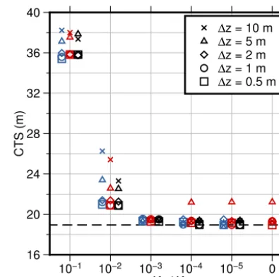
Figure 3. Comparison of simulated steady-state CTS positions for
different values of the temperate ice conductivity in Experiment B. The different models are shown as: TIM-FD3(blue), ISSM (red) and COMice (black). Results of different models are slightly shifted on thex-axis to not overlay each other. The dashed black line indi-cates the CTS position of the analytical solution derived forK0=0.
After ∼1000 years the cold signal from the surface reaches the base and melting starts to decrease until the tem-perature gradient in the overlying ice does not allow for fur-ther melting and refreezing sets in. All models agree well with the analytical solution. The COMice solution is some-times slightly below the analytical solution because of the very large time steps. The transition between melting and freezing occurs after∼4684.7 years in the analytical solu-tion. Model simulations show this transition at a comparable modelled time.
All model results clearly reveal reversibility: after the whole simulation period of 300 ka, the models return to the initial steady state at the end of phase I.
5.2 Experiment B
Here, model results of the steady-state simulations of exper-iment B are compared to the analytical solution given in Ap-pendix A2. For TIM-FD3 and COMice the steady state is assumed after 1000 model years, while in ISSM a thermal steady-state solver is applied. The final steady-state CTS po-sitions for all simulations are shown in Fig. 3.
so-T. Kleiner et al.: Enthalpy benchmark experiments 223 lution. The models have approximately the same spread for
the different vertical resolutions. The spread of the CTS po-sition is smallest for CR=10−3independent of the applied
model. Compared to ISSM, TIM-FD3 and COMice imple-mentations do not allow for solving the caseK0=0 as in the
analytical solution.
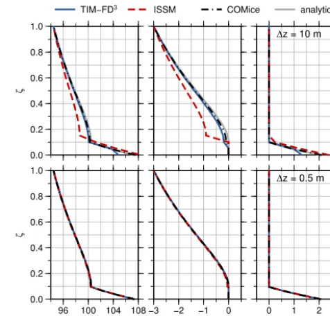
The steady-state enthalpy profiles and the corresponding temperature and moisture profiles are shown in Fig. 4 to-gether with the analytical solution given in Appendix A2. The profiles are shown for the lowest (10 m) and highest (0.5 m) vertical resolution and the lowest conductivity ratio CR=10−5 used by all models. The results of all models agree well with the analytical solution for high resolutions. At coarser resolutions the simulated enthalpy profiles differ noticeably from the analytical solution. In the following we compare enthalpy differences as1E=Eanalytic−Esimulated.
In the ISSM simulation with the coarsest resolution (1z=10 m), the enthalpy differs from the analytical solution by∼1720 J kg−1close to the CTS. This results in a temper-ature difference of ∼0.9◦C in the cold ice part. TIM-FD3 and COMice reveal also a lower enthalpy at the cold side of the CTS compared to the analytical solution, but only to a minor extent (TIM-FD3:∼0.2◦C, COMice:∼0.1◦C). Note that the analytical solution only holds forK0=0, thus small
differences are expected here.
As the method chosen for interpolating heat conductivities in ISSM strongly favours the lower value, a quasi-isolating layer thicker than in the analytical solution is artificially cre-ated. Thus, heat flux into the upper cold ice column de-creases, and that column cools. Vice versa, excess heat is accumulated in the lower temperate ice column, such that this part of the ice column heats up. The result is a nega-tive temperature and posinega-tive water fraction offset. It scales with vertical mesh resolution, but stays detectable even on the highest mesh resolution tested here.
In the TIM-FD3 simulation with the coarsest resolution (1z=10 m), the enthalpy difference 1E is largest at the base (∼2530 J kg−1). As the base is temperate, this differ-ence in the enthalpy corresponds to a differdiffer-ence in the basal water content of ∼0.8 %. With this resolution the temper-ate ice layer needs to be resolved within the lowermost three grid points. The slope in the profile is caused by second-order one-sided discretization (e.g. Payne and Dongelmans, 1997) of the basal boundary condition (Eq. 6) in TIM-FD3. Com-pared to the FE models neither strain heating nor transport of heat is considered for basal grid nodes.
With increasing vertical resolution the maximum devia-tion from the analytical soludevia-tion decreases for all models. For the highest resolution (1z=0.5 m) and CR=10−5 the maximum differences are ∼150 J kg−1, ∼100 J kg−1 and
∼10 J kg−1for TIM-FD3, ISSM and COMice, respectively. The differences remain positive, thus the enthalpy is slightly underestimated. Only ISSM is able to perform the experi-ment withK0=0 as in the analytical solution, but the
max-imum enthalpy difference does not further decrease. As
ex-Discussion
P
ap
er
|
Discussion
P
ap
er
|
Discussion
P
ap
er
|
Discussion
P
ap
er
|
0.0 0.2 0.4 0.6 0.8 1.0
ζ
96 100 104 108
E (103 J kg−1)
−3 −2 −1 0
T (°C)
0 1 2 3
ω (%)
∆z = 0.5 m
0.0 0.2 0.4 0.6 0.8 1.0
ζ
TIM−FD3 ISSM COMice analytical
∆z = 10 m
Figure 4.Simulated steady state profiles of the enthalpy,E, the temperature,T, and the water
content,ωfor TIM-FD3(blue), ISSM (red) and COMice (black) compared to the analytical solution
(gray).ζ=z/His the normalised vertical coordinate. The vertical resolution is∆z= 10 m(upper
row) and∆z= 0.5 m(lower row),CR=K0/Kc= 10−5. In the lower row the model results overlay
the analytical solution.
32
Figure 4. Simulated steady-state profiles of the enthalpyE, the tem-peratureTand the water contentωfor TIM-FD3(blue), ISSM (red) and COMice (black) compared to the analytical solution (grey).
ζ=z/H is the normalized vertical coordinate. The vertical res-olution is 1z=10 m (upper row) and 1z=0.5 m (lower row), CR=K0/Kc=10−5. In the lower row the model results overlay
the analytical solution.
pected from Eq. (11) all models show small enthalpy gradi-ents at the cold side of the CTS.
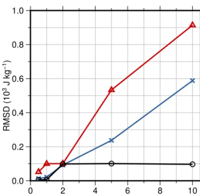
The observed order of accuracy measured as the root-mean-square deviation (RMSD) to the analytical solution has been obtained in the series of vertical mesh refinements from1z=10 to 0.5 m and is shown in Fig. 5. The models TIM-FD3and ISSM show approximately first-order conver-gence as1z→0, while in COMice the RMSD drops only for1zbelow 2 m. The finite difference discretization scheme in TIM-FD3is formally second-order accurate in space (and time) and the finite element models ISSM and COMice use linear basis functions, thus one would expect second-order convergence as1z→0 for smooth problems. However, this is not the case here, since the observed order of accuracy de-pends on the strength of discontinuities (conductivity ratio between cold and temperate ice) and on the CTS implemen-tation details.
6 Discussion
tem-224 Discussion T. Kleiner et al.: Enthalpy benchmark experiments
P
ap
er
|
Discussion
P
ap
er
|
Discussion
P
ap
er
|
Discussion
P
ap
er
|
0.0 0.2 0.4 0.6 0.8 1.0
RMSD (10
3 J kg
−1
)
0 2 4 6 8 10
∆z (m)
Figure 5.The root-mean-square deviation (RMSD) of the model results to the analytical solution (Experiment B) for different vertical grid resolutions∆z. Model results for TIM-FD3(blue crosses), ISSM (red triangles) and COMice (black circles) are obtained for the lowest conductivity ratioCR= K0/Kc= 10−5applied to all models.
33
Figure 5. The root-mean-square deviation (RMSD) of the model
results to the analytical solution (Experiment B) for different verti-cal grid resolutions1z. Model results for TIM-FD3(blue crosses), ISSM (red triangles) and COMice (black circles) are obtained for the lowest conductivity ratio CR=K0/Kc=10−5 applied to all
models.
perate ice layer at the base, the insulating boundary condition (Eq. 6) could not be tested.
Beside the test of the implementation of the boundary con-ditions, this experiment addresses the importance of a basal water layer. Although the surface temperature changes, the basal temperature is kept at pressure melting point as long as a basal water layer exists. The amount of water at the base is crucial for the temperatures in the ice, because it acts as an energy buffer. It slows down the response of basal temper-atures to surface cooling. The water layer thicknesses sim-ulated here are unrealistically high compared to conditions under real ice masses. More realistic simulations would re-quire a subglacial hydrology model, but this is beyond the scope of this paper.
Experiment B addresses whether the models are able to re-produce the steady-state analytical solution for certain poly-thermal conditions including advection, diffusion and strain heating. The models agree well with the analytical solu-tion for K0→0, if the vertical resolution is high. All
mod-els meet the transition conditions for the melting CTS, al-though no explicit boundary conditions are implemented. An adequate treatment of the abrupt change of conductivity at the CTS in the numerical discretization scheme is required to achieve this behaviour. The usage of an arithmetic mean (TIM-FD3) or a Heaviside as well as a smoothed Heaviside function (COMice) for the conductivity jump leads to oscil-lations in the enthalpy solution that are visible e.g. in a time-varying CTS position. Consequently, no steady-state solution is reached under these conditions. The harmonic mean ap-proach of Patankar (1980, chap. 4.2.3) for the conductivity
(TIM-FD3and ISSM) leads to a continuous heat flux at the CTS and violates the condition of Eq. (11) (non-continuous). Nevertheless, the harmonic mean strongly favours the lower conductivityK0for small ratios CR=K0/Kcand this leads
to the apparent jump in∂E/∂z.
TIM-FD3tends to underestimate the water content at the base of a temperate ice layer. This would result in stiffer ice at the base. In typical applications of the model the vertical layers are not equidistant as in this study, but refined towards the base. We therefore expect only a minor influence on the velocity field. ISSM simulations underestimate the tempera-ture in the cold part accompanied by an overestimation of the water content in the basal temperate layer at coarse resolu-tion. Implications for the overall stiffness are hard to obtain. Ice would deform more in the temperate part at the base, but less in the cold part above.
The understanding of moisture transport in the temperate ice is poor. If the latent heat flux can be represented as in As-chwanden et al. (2012), then it is crucial to consider the as-sumption made on the chosen value ofK0. Simulations with
a relatively high value ofK0would lead to a much thicker
temperate ice layer in contrast to simulations whereK0≈0.
Stable numerical solutions could be obtained for temper-ate ice diffusivities in the chosen range of K0≈10−4 to
10−8kg m−1s−1and 0 for ISSM. The lower bound is there-fore several magnitudes lower thanK0=10−4kg m−1s−1as
the lowest value possible for a stable solution in Aschwanden and Blatter (2009). If one assumes a vanishing latent heat flux in the temperate part of a glacier, we would recommend us-ing a value ofK0≈10−6kg m−1s−1(CR=10−3). For this
value the CTS positions of all models are close to the an-alytical solution and show the smallest spread with varying vertical resolutions (Fig. 3).
The evolution equation for the enthalpy field is similar to the temperature evolution equation already implemented in thermomechanically coupled ice sheet models. Therefore an enthalpy scheme allows one to convert so-called “cold ice” models into polythermal ice models with only minor mod-ifications, but with the restriction of melting conditions at the CTS. The question of whether exclusive melting condi-tions at the CTS are valid in an ice sheet is not conclusive. At least simulations of the Greenland Ice Sheet based on a two-layer front-tracking scheme performed with the poly-thermal ice model SICOPOLIS indicate that freezing con-ditions are relatively rare (Greve, 1997a, b). In the most recent version of SICOPOLIS the enthalpy scheme of As-chwanden et al. (2012) and a modified version of this scheme have been implemented as conventional one-layer enthalpy scheme and one-layer melting CTS scheme, respectively (Blatter and Greve, 2014). Thus comparisons to the two-layer front-tracking scheme can be performed for continental-scale ice sheets in the future.
knowl-T. Kleiner et al.: Enthalpy benchmark experiments 225 edge on the rheology of temperate ice, the current
experi-mentally based relationship for the flow rate factor is only valid for water contents up to 1 % (Duval, 1977; Lliboutry and Duval, 1985). However, actual water contents found in temperate and polythermal glaciers are sometimes substan-tially larger (up to 5 %, Bradford and Harper, 2005). The ad-vantage of deriving the water content by solving numerically for the enthalpy is limited by the use of a flow rate factor with a restricted validity range. Consequently, deformation experiments with temperate ice are urgently needed.
7 Conclusions
The proposed numerical experiments provide tests for the enthalpy implementation in numerical ice sheet models. All models applied here (TIM-FD3, ISSM, COMice) are able to perform these experiments successfully and agree to the ana-lytical solutions. The enthalpy scheme determines the cold– temperate transition surface (CTS) and the vertical enthalpy profile in a polythermal glacier correctly without the need of tracking the CTS explicitly and applying additional condi-tions at this internal boundary. This is in particular the case for high vertical resolution for all three models. TIM-FD3 and COMice also perform well for low vertical resolution, while the ISSM solution shows a significant enthalpy differ-ence to the analytical solution although the analytical CTS position is met. There is a clear need for an empirical de-termination of the temperate ice conductivityK0and an
226 T. Kleiner et al.: Enthalpy benchmark experiments
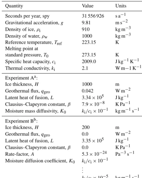
Table A1. Constants and model parameters used.
Quantity Value Units
Seconds per year, spy 31 556 926 s a−1 Gravitational acceleration,g 9.81 m s−2
Density of ice,ρi 910 kg m−3
Density of water,ρw 1000 kg m−3
Reference temperature,Tref 223.15 K Melting point at
standard pressure,T0 273.15 K
Specific heat capacity,ci 2009.0 J kg−1K−1
Thermal conductivity,ki 2.1 W m−1 K−1
Experiment Aa:
Ice thickness,H 1000 m
Geothermal flux,qgeo 0.042 W m−2
Latent heat of fusion,L 3.34×10⁵ J kg−1 Clausius–Clapeyron constant,β 7.9×10⁻⁸ K Pa−1 Moisture mass diffusivity,K0 ki/ci×10−1 kg m−1s−1
Experiment Bb:
Ice thickness,H 200 m
Geothermal flux,qgeo 0.0 W m−2
Latent heat of fusion,L 3.35×10⁵ J kg−1 Clausius–Clapeyron constant,β 0.0 K Pa−1
Rate-factor,A 5.3×10⁻²⁴ Pa−3s−1
Moisture diffusion coefficient,K0 ki/ci×10−1 .
. .
ki/ci×10−5 kg m−1s−1
aAschwanden et al. (2012);bGreve and Blatter (2009).
Appendix A: Analytical solutions A1 Basal melt rate in Experiment A
To derive the basal melt rate for phase IIIa of Experiment A it is assumed that the temperature is in steady state at the end of the warming phase II. For this set-up Eq. (2) simplifies to the one-dimensional form
ρi ∂E
∂t = ∂ ∂z
Kc
∂E ∂z
. (A1)
We have only cold ice conditions in the interior of the ice body andKcas well asρiare constants. Based on the
trans-fer rules in Eq. (1), Eq. (A1) can be written as an evolution equation for the temperature:
∂T ∂t =κ
∂2T
∂z2 andκ= ki ρici
. (A2)
We determine the evolution ofT (z,t) starting from the initial condition (steady-state temperature profile of phase II) T (z,0)=T0(z)=Tpmp+ Ts,w−Tpmpz/H (A3)
and Dirichlet conditions at the upper and lower surface
T (H, t )=Ts,wandT (0, t )=Tpmp. (A4)
The basal temperature is kept at pressure melting point by the basal water layer (Eq. 7). Solutions of the heat equations can be found by separation of variables and Fourier analysis and require homogeneous boundary conditions. Therefore, the temperature deviation2is used instead ofT, thus
T (z, t )=Teq(z)+2(z, t ), (A5)
where the steady-state profile for this set-up is again a linear Teq(z)=Tpmp+ Ts,c−Tpmpz/H. (A6)
Substitution of Eq. (A5) into Eq. (A2) and application of the steady-state solutionTeq(z)implies that2(z,t) satisfies the
homogeneous heat equation ∂2
∂t =κ ∂22
∂z2 (A7)
with homogeneous Dirichlet boundary conditions,
2(0, t )=2(H, t )=0 fort >0 (A8) and the initial condition
2(z,0)=T0(z)−Teq(z)for 0≤z≤H. (A9)
The solution of Eqs. (A7)–(A9) for2can be obtained us-ing the method of separation of variables and leads to (e.g. Dubin, 2003)
2(z, t )= ∞
X
n=1
Aneλntsin nπ z
H ,
whereλn= −κ nπ
H 2
. (A10)
Setting t=0 the Fourier coefficients An can be found by matching the initial condition Eq. (A9):
2(z,0)= ∞
X
n=1 Ansin
nπ z
H =T0(z)−Teq(z). (A11) Thus for the Fourier sine series, the coefficientsAn are de-termined as
An= 1 H
H Z
0
T0(z)−Teq(z)sin nπ z
H dz. (A12)
Inserting the initial condition (Eq. A3) and the steady-state profile (Eq. A6) into Eq. (A12) leads to
An=(−1)n+1
2 Ts,w−Ts,c
T. Kleiner et al.: Enthalpy benchmark experiments 227 Based on the analytical solution of the temperature profile
(Eq. A10) the basal melt rate (Eq. 8) is
ab=
qgeo−qi
ρL =
1 ρL
qgeo+k
∂T ∂z|z=0
, (A14)
where ∂T
∂z|z=0= ∂Teq(z)
∂z |z=0+
∂2(z, t ) ∂z |z=0
=Ts,c−Tpmp
H +
∞
X
n=1 nπ
H Ane
λnt. (A15)
The sum is evaluated up ton=25 to produce the analytical solution shown in Fig. 2.
A2 Analytical solution Experiment B
The following derivation of the analytical solution to experi-ment is a modification of the derivation of the “parallel-sided polythermal slab” provided by Greve and Blatter (2009). Un-der the assumptions given there and the variable transform z=ζ H, the enthalpy field Eq. (2) reduces to
D∂
2E ∂ζ2 +M
∂E
∂ζ = −K(1−ζ )
4, ifE < E
pmp (A16)
M∂E
∂ζ = −K(1−ζ )
4, else. (A17)
Here,
D=Ki
ρ ,M=H a
⊥ s ,K=
2A
ρ (ρgsinγ )
4H6. (A18)
Let E+ be a solution of Eq. (A16) and E− a solution to Eq. (A17). Then the enthalpy solution for the entire ice col-umn is given byE=E−I[0,ζm)+E
+
I[ζm,1], whereζmis the
position of the CTS.
At the CTS the continuity condition for the enthalpy Eq. (10) holds and due to the neglect of water conductiv-ity in temperate ice the right-hand side of Eq. (11) is zero. A solutionE+to Eq. (A16) is given by a solution to the homo-geneous differential equationEh associated with Eq. (A16)
and a particular solutionEp:
E+=Eh+Ep,with (A19)
Eh(ζ )=c1e−Mζ /D+c2,and (A20) Ep(ζ )=
5 X
k=1
akζk. (A21)
The coefficientsa1, . . . ,a5ofEpcan be found by balancing
powers in Eq. (A16) (see Greve and Blatter, 2009). The three remaining unknowns,c1,c2andζm, can now be derived from
the conditions at the CTS (Eqs. 10 and 11) and the given surface enthalpy. InsertingE+yields
Es=c1e−M/D+c2+ 5 X
k=1
ak (A22)
Epmp=c1e−Mζm/D+c2+ 5 X
k=1
akζmk (A23)
0= −c1
M
De
−Mζm/D+
5 X
k=1
kakζmk−1. (A24)
With c1 from Eq. (A24) and c2 from Eq. (A22), then
Eq. (A23) becomes an implicit definition forζm, whose root
can be determined using a numerical solver. Thenc1andc2
follow accordingly.
A solutionE−for the temperate ice part can be found by integrating the temperate version of Eq. (A17) directly.E− is then fully determined by Eq. (11):
E−(ζ )=Epmp+
K
5M
(1−ζ )5−(1−ζm)5
228 T. Kleiner et al.: Enthalpy benchmark experiments
Acknowledgements. The authors would like to thank H. Blatter,
R. Greve, F. J. Navarro, J. Otero and F. Ziemen for fruitful discussions on enthalpy and ice sheet models. We acknowledge the support of the ISSM developer team (E. Larour, H. Seroussi and M. Morlighem) for the implementation of the enthalpy formulation in ISSM.
Edited by: F. Pattyn
References
Aschwanden, A. and Blatter, H.: Mathematical modeling and nu-merical simulation of polythermal glaciers, J. Geophys. Res., 114, F01027, doi:10.1029/2008JF001028, 2009.
Aschwanden, A., Bueler, E., Khroulev, C., and Blatter, H.: An en-thalpy formulation for glaciers and ice sheets, J. Glaciol., 58, 441–457, doi:10.3189/2012JoG11J088, 2012.
Blatter, H. and Greve, R.: Comparison and verification of enthalpy schemes for polythermal glaciers and ice sheets with a one-dimensional model, Polar Science, submitted, preprint at ArXiv E-Prints, arXiv:1410.6251, 2014.
Blatter, H. and Hutter, K.: Polythermal conditions in Arctic glaciers, J. Glaciol., 37, 261–269, 1991.
Bradford, J. H. and Harper, J. T.: Wave field migration as a tool for estimating spatially continuous radar velocity and water content in glaciers, Geophys. Res. Lett., 32, L08502, doi:10.1029/2004GL021770, 2005.
Bueler, E., Lingle, C. S., Kallen-Brown, J. A., Covey, D. N., and Bowman, L. N.: Exact solutions and the verification of numerical models for isothermal ice sheets, J. Glaciol., 51, 291–306, 2005. Bueler, E., Brown, J., and Lingle, C. S.: Exact solutions to the thermomechanically coupled shallow-ice approxima-tion: effective tools for verification, J. Glaciol., 53, 499–516, doi:10.3189/002214307783258396, 2007.
Dubin, D.: Numerical and Analytical Methods for Scientists and Engineers Using Mathematica, Wiley, Hoboken, New Jersey, USA, 656 pp., 2003.
Duval, P.: The role of the water content on the creep rate of poly-crystalline ice, International Association of Hydrological Sci-ences Publication 118, Symposium on Isotopes and Impurities in Snow and Ice, Grenoble, 29–33, 1977.
Fowler, A. C.: On the transport of moisture in poly-thermal glaciers, Geophys. Astro. Fluid, 28, 99–140, doi:10.1080/03091928408222846, 1984.
Glen, J. W.: The Creep of Polycrystalline Ice, P. Roy. Soc. Lond. A, 228, 519–538, 1955.
Greve, R.: Application of a polythermal three-dimensional ice sheet model to the Greenland Ice Sheet: response to steady-state and transient climate scenarios, J. Climate, 10, 901–918, 1997a. Greve, R.: A continuum-mechanical formulation for shallow
poly-thermal ice sheets, Philos. T. Roy. Soc. Lond., 355, 921–974, 1997b.
Greve, R. and Blatter, H.: Dynamics of ice sheets and glaciers, in: Advances in Geophysical and Environmental Mechan-ics and MathematMechan-ics, Springer, Berlin, Heidelberg, 287 pp., doi:10.1007/978-3-642-03415-2, 2009.
Hindmarsh, A. C., Brown, P. N., Grant, K. E., Lee, S. L., Serban, R., Shumaker, D. E., and Woodward, C. S.: SUNDIALS: Suite of Nonlinear and Differential/Algebraic Equation Solvers, ACM T. Math. Software, 31, 363–396, doi:10.1145/1089014.1089020, 2005.
Hutter, K., Blatter, H., and Funk, M.: A model computation of mois-ture content in polythermal glaciers, J. Geophys. Res.-Sol. Ea., 93, 12205–12214, doi:10.1029/JB093iB10p12205, 1988. Huybrechts, P., Payne, T., Abe-Ouchi, A., Calov, R., Fabre, A.,
Fas-took, J. L., Greve, R., Hindmarsh, R. C. A., Hoydal, O., Jo-hannesson, T., MacAyeal, D. R., Marsiat, I., Ritz, C., Verbit-sky, M. Y., Waddington, E. D., and Warner, R.: The EISMINT benchmarks for testing ice-sheet models, Ann. Glaciol., 23, 1– 12, 1996.
Kleiner, T. and Humbert, A.: Numerical simulations of major ice streams in western Dronning Maud Land, Antarctica, un-der wet and dry basal conditions, J. Glaciol., 60, 215–232, doi:10.3189/2014JoG13J006, 2014.
Larour, E., Seroussi, H., Morlighem, M., and Rignot, E.: Continen-tal scale, high order, high spatial resolution, ice sheet modeling using the Ice Sheet System Model (ISSM), J. Geophys. Res., 117, F01022, doi:10.1029/2011JF002140, 2012.
Lliboutry, L. A. and Duval, P.: Various isotropic and anisotropic ices found in glaciers and polar ice caps and their corresponding rheologies, Ann. Geophys.-Italy, 3, 207–224, 1985.
Notz, D. and Worster, M. G.: A one-dimensional en-thalpy model of sea ice, Ann. Glaciol., 44, 123–128, doi:10.3189/172756406781811196, 2006.
Patankar, S. V.: Numerical Heat Transfer and Fluid Flow, McGraw-Hill, New York, 1980.
Pattyn, F., Schoof, C., Perichon, L., Hindmarsh, R. C. A., Bueler, E., de Fleurian, B., Durand, G., Gagliardini, O., Gladstone, R., Goldberg, D., Gudmundsson, G. H., Huybrechts, P., Lee, V., Nick, F. M., Payne, A. J., Pollard, D., Rybak, O., Saito, F., and Vieli, A.: Results of the Marine Ice Sheet Model Intercomparison Project, MISMIP, The Cryosphere, 6, 573–588, doi:10.5194/tc-6-573-2012, 2012.
Payne, A. J. and Dongelmans, P. W.: Self-organization in the ther-momechanical flow of ice sheets, J. Geophys. Res., 102, 12219– 12233, doi:10.1029/97JB00513, 1997.
Rückamp, M., Blindow, N., Suckro, S., Braun, M., and Humbert, A.: Dynamics of the ice cap on King George Island, Antarctica: field measurements and numerical simulations, Ann. Glaciol., 51, 80–90, doi:10.3189/172756410791392817, 2010.
Seroussi, H., Morlighem, M., Rignot, E., Khazendar, A., Larour, E., and Mouginot, J.: Dependence of century-scale projections of the Greenland ice sheet on its thermal regime, J. Glaciol., 59, 1024– 1034, doi:10.3189/2013JoG13J054, 2013.
Spalding, D. B.: A novel finite difference formulation for differen-tial expressions involving both first and second derivatives, Int. J. Numer. Meth. Eng., 4, 551–559, doi:10.1002/nme.1620040409, 1972.