Earth Syst. Sci. Data, 2, 247–260, 2010 www.earth-syst-sci-data.net/2/247/2010/ doi:10.5194/essd-2-247-2010
©Author(s) 2010. CC Attribution 3.0 License.
History
ofGeo- and Space
Sciences
Open
Access
Advances
in Science & ResearchOpen Access Proceedings
Open Access Earth System
Science
Data
Open Access Earth SystemScience
Data
D iscussionsDrinking Water
Engineering and Science
Open Access
Drinking Water
Engineering and Science Discussions O pen Acc es s
Social
Geography
Open Access D iscussionsSocial
Geography
Open AccessAn improved Antarctic dataset for high resolution
numerical ice sheet models (ALBMAP v1)
A. M. Le Brocq1,2, A. J. Payne3, and A. Vieli1
1Department of Geography, Durham University, Durham, UK
2Geography, College of Life and Environmental Sciences, University of Exeter, Exeter, UK 3Bristol Glaciology Centre, School of Geographical Sciences, University of Bristol, Bristol, UK
Received: 14 June 2010 – Published in Earth Syst. Sci. Data Discuss.: 28 June 2010 Revised: 1 October 2010 – Accepted: 5 October 2010 – Published: 11 October 2010
Abstract. The dataset described in this paper (ALBMAP) has been created for the purposes of high-resolution numerical ice sheet modelling of the Antarctic Ice Sheet. It brings together data on the ice sheet configuration (e.g. ice surface and ice thickness) and boundary conditions, such as the surface air temperature, accumulation and geothermal heat flux. The ice thickness and basal topography is based on the BEDMAP dataset (Lythe et al., 2001), however, there are a number of inconsistencies within BEDMAP and, since its release, more data has become available. The dataset described here addresses these inconsistencies, including some novel interpolation schemes for sub ice-shelf cavities, and incorporates some major new datasets. The inclusion of new datasets is not exhaustive, this considerable task is left for the next release of BEDMAP, however, the data and procedure documented here provides another step forward and demonstrates the issues that need addressing in a continental scale dataset useful for high resolution ice sheet modelling. The dataset provides an initial condition that is as close as possible to present-day ice sheet configuration, aiding modelling of the response of the Antarctic Ice Sheet to various forcings, which are, at present, not fully understood.
1 Introduction
There is a great deal of uncertainty over the potential con-tribution of the Antarctic Ice Sheet to sea level rise over the next century. The 2007 IPCC (Intergovernmental Panel on Climate Change) report (see chapter 10: Meehl et al., 2007), for example, did not include the potential contribu-tion to sea level change from retreat of the Antarctic Ice Sheet because of the uncertainty over its response to climate change. In order to reduce this uncertainty, high-resolution numerical ice sheet models (grid resolution of≤5 km com-pared to 20–50 km previously), with higher-order physics, are needed to reproduce the present day behaviour of the ice sheet and predict the response of the ice sheet into the fu-ture. Advances are currently being made in developing high-resolution, higher-order models (e.g. Pattyn, 2002; Price et al., 2007; Hubbard et al., 2009). There is also particular focus on representing grounding line (where the ice changes from being grounded to floating) retreat/advance (e.g. Schoof,
Correspondence to: A. M. Le Brocq
2007; Pollard and DeConto, 2009). However, the results from these models are only as good as the data that are in-put; in particular the elevation of the bed and bathymetry at the grounding line.
It is now possible to download a community ice sheet model (e.g. Elmer/Ice, Glimmer-CISM, SICOPOLIS), mak-ing ice sheet modellmak-ing accessible for many purposes, how-ever, without adequate data it is difficult to utilise such mod-els. Whilst the BEDMAP dataset (Lythe et al., 2001) was a step forward when it was created, providing data on ice thickness, surface and bed elevations, there are a number of inconsistencies within the dataset (see Sect. 3). These incon-sistencies cause difficulties for ice sheet models, particularly those which use the present day configuration as a starting point. Also since the release of BEDMAP, more data have become available regarding both the ice thickness and sur-face elevation.
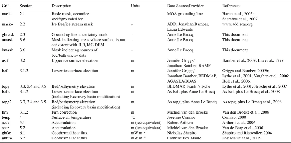
Table 1.List of datasets included and source.
Grid Section Description Units Data Source/Provider References
mask 2.1 Basic mask, ocean/ice
shelf/grounded ice
– MOA grounding line Haran et al., 2005;
Scambos et al., 2007
mask+ 2.2 Ice free/ice stream mask – ADD, Jonathan Bamber,
Laura Edwards
www.add.scar.org
glmask 2.3 Grounding line uncertainty mask – Anne Le Brocq This document
umask 3.6 Mask indicating areas where surface is not
consistent with JLB/JAG DEM
– Anne Le Brocq This document
bmask 3.6 Mask indicating sources of
bed/bathymetry data
– Anne Le Brocq This document
usrf 3.2 Upper ice surface elevation m Jennifer Griggs/
Jonathan Bamber, RAMP
Bamber et al., 2009; Liu et al., 1999
lsrf 3.1.2 Lower ice surface elevation m Jennifer Griggs/
Jonathan Bamber, BEDMAP,
AGASEA/BBAS
Griggs and Bamber, 2009b;
Lythe et al., 2001; Vaughan et al., 2006; Holt et al., 2006.
topg 3.3, 3.4 and 3.5 Bed/bathymetry elevation m BEDMAP, Frank Nitsche Lythe et al., 2001; Nitsche et al., 2007
lsrf2 3.1.2 Lower ice surface elevation
(including Recovery basin modification)
m As lsrf, plus Anne Le Brocq As lsrf, plus Le Brocq et al., 2008
topg2 3.3, 3.4 and 3.5 Bed/bathymetry elevation
(including Recovery basin modification)
m As topg, plus Anne Le Brocq As topg, plus Le Brocq et al., 2008
firn 3.1.2 Firn correction m Michiel van den Broeke Van den Broeke et al., 2008
temp 4 Surface air temperature ◦
C Josefino Comiso Comiso, 2000
acca 5.1 Accumulation m (ice equivalent) Robert Arthern Arthern et al., 2006
accr 5.2 Accumulation m (ice equivalent) Michiel van den Broeke Van de Berg et al., 2006
ghfsr 6.1 Geothermal heat flux mW m−2 Nicholas Shapiro Shapiro and Ritzwoller, 2004
ghffm 6.2 Geothermal heat flux mW m−2 Cathrine Fox Maule Fox Maule et al., 2005
means incorporates all the new data available. This consid-erable task is left for a “BEDMAP2”, (an updated version of BEDMAP), however, the processing carried out in this docu-ment illustrates the requiredocu-ments of a dataset for the purpose of high resolution ice sheet modelling, and bridges the gap until BEDMAP2 is published.
Whilst the ice sheet configuration datasets described here may be used for other purposes, the user should be aware that the focus of the data preparation was on assembling a dataset suitable for ice sheet modelling. For example, no claims are made about the accuracy of the sub ice-shelf interpolation, only that it is a “best guess” and it allows the ice shelf to float. This paper does not attempt to consider or quantify dataset errors, the reader is referred to original references for this.
The dataset presented here also includes the most up-to-date versions of boundary conditions required to drive an Antarctic Ice Sheet model, namely, surface air temperature, accumulation and geothermal heat flux, and also a number of masks delineating the different parts of the ice sheet. This paper describes the data processing carried out to produce the final datasets: firstly, the masks and ice sheet configuration datasets are described (Sects. 2 and 3 respectively), then the surface air temperature (Sect. 4), the accumulation (Sect. 5) and finally the geothermal heat flux (Sect. 6).
1.1 Dataset overview and format
The dataset is available at doi:10.1594/PANGAEA.734145. Table 1 lists the data available in the overall dataset and pro-vides an indication of the various sources of data. For a full description see the relevant section in this document.
The data are provided in a netcdf data format, see http: //www.unidata.ucar.edu/software/netcdf/for more details of this data format. Many tools are available to convert the data. For example, ncdump, ncks, and nco can be used to extract ASCII data, Ncview, Panoply, and GMT could be used to view the data and mathematical operations can applied with NCO or GMT. In addition some commercial programs are also able to interpret netcdf files, tools to convert the data are available, for example, in Matlab and ArcGIS (9.2 onwards). The data are on a 5 km resolution grid, in a Polar Stereo-graphic Projection (Central Meridian, 0◦, Standard Parallel,
Table 2.Mask values.
Mask file Value Description mask 0 Ocean mask 1 Grounded ice mask 2 Ice shelf
mask+ 0 Non ice free/ice stream mask+ 3 Ice free
mask+ 4 Ice stream (>250 m yr−1)
glmask 0 Non “ice plain” glmask 5 “Ice plain”
2 Masks
2.1 “mask”
The basic mask delineates ocean, grounded ice sheet and ice shelf regions of Antarctica. The mask is derived from the MOA (Mosaic of Antarctica) coastline shapefiles (Ha-ran et al., 2005; Scambos et al., 2007). The ice thickness dataset (described later in Sect. 3.1.3) is composed of two separate datasets: the grounded ice sheet thickness, largely from BEDMAP, and ice shelf thickness, derived from the surface elevation and an assumption of hydrostatic equilib-rium. In order to create a smooth join between the grounded and floating ice thickness datasets, a number of iterations are carried out where the mask (more specifically, the ground-ing line location) is modified to ensure the best join between the two datasets. Small changes are made away from ice stream grounding line areas, allowing for a one grid cell width smoothing boundary (see Sect. 3.1.3). Larger changes are made at a number of ice stream grounding zone locations, where the MOA grounding line is believed to be inaccurate. The areas of major change are discussed in Sect. 2.3 below.
Three islands were found to be missing from the original MOA dataset (Smyley Island and Case Island at the western end of George VI Ice Shelf, and Sherman Island incorporated in the Abbott Ice Shelf), these were added by digitising their extent from the original MOA image. The mask values are given in Table 2.
The mask was then modified to make it “modelling friendly”, i.e. by removing small ice shelves (1 or 2 cells), and islands only one grid cell wide.
2.2 “mask+”
The purpose of the “mask+” mask is to provide extra infor-mation on the ice sheet, beyond that provided in the basic mask. It indicates terrestrial regions that are currently ice free (see Sect. 2.2.1 below) and ice stream regions, here de-fined by velocities over 250 m yr−1 (see Sect. 2.2.2 below).
Mask+also contains the base values from “mask”.
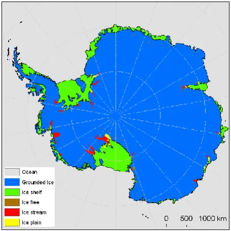
Figure 1.Combination of mask, mask+and glmask.
2.2.1 Ice free areas
The ice free regions were derived from the ADD (Antarc-tic Digital Database) “rock” polygon coverage. The polygon coverage was converted to the 5 km grid, based on the per-centage of the cell which is ice free (rock). A threshold of 33% of the cell being ice free was chosen, based on the re-sulting 5 km mask. Hence the 5 km ice free mask does not include all areas which are ice free, only those which cover a certain area.
2.2.2 Ice stream areas
The ice stream regions were derived from a combined map of InSAR velocities (Edwards, 2008). The InSAR velocity map does not cover all regions, hence some ice streams have been supplemented by balance velocities. The mask only in-cludes the “major” ice streams, some small outlet glaciers are not coherent enough at a 5 km resolution, so have not been included (Fig. 1). Therefore the mask should only be consid-ered indicative rather than definitive.
2.3 “glmask”
is not the “break of slope”, hence, the MOA mask is often a long way (10 s of km) inland from where it is believed to be (notably Pine Island Glacier, Slessor Glacier). The ADD grounding line is, therefore, more reliable in some ice stream regions (though generally much less reliable than MOA in other areas).
3 Ice sheet configuration
As mentioned in the introduction, the BEDMAP dataset pro-vides information on the bed topography, bathymetry and ice thickness. However it contains a large number of in-consistencies, (e.g. bed plus ice thickness not equal to mea-sured surface) and when a flotation calculation is carried out, it does not provide a grounding line consistent with obser-vations. It is the aim of this section to produce a dataset that is free of these inconsistencies, suitable for initialising a numerical model for the present day ice sheet configura-tion. The following discussion outlines the important factors which need to be considered.
Firstly, at the most basic level, it is important that all the configuration datasets are self consistent, i.e. that if the sur-face elevation is derived from the bed and ice thickness, then it is consistent with the provided surface elevation.
Secondly, it is critical that if the mask says the ice is grounded, then it is grounded and likewise for floating ice. BEDMAP has a large number of ice shelf areas which be-come grounded due to poor sub ice-shelf interpolation. If the ice surface is derived by adding the ice thickness to the basal topography in areas which become grounded, then this will introduce a large number of grounded “islands” into the ice shelf areas.
Thirdly, around ice stream grounding zones, it is important that no modifications affect the ice sheet surface, e.g. chang-ing the ice shelf thickness will change the resultchang-ing ice sur-face from a flotation calculation. The ice sursur-face derived from any flotation calculation must be consistent with the measured surface, hence, in the ALBMAP dataset, the ice thickness in the ice shelf areas is derived from the ice surface and a firn correction. Any flotation calculation must include the firn correction and use the densities given here to ensure the ice sheet surface remains consistent. Otherwise, spurious bumps will appear, which will be highly noticeable in low slope ice stream regions.
Finally, it is also important that there are no false or large gradients in the ice surface, thickness or bed/bathymetry, as can arise when a number of datasets are combined. The con-sequence of this would be unfeasibly large gravitational driv-ing stress (and hence velocities).
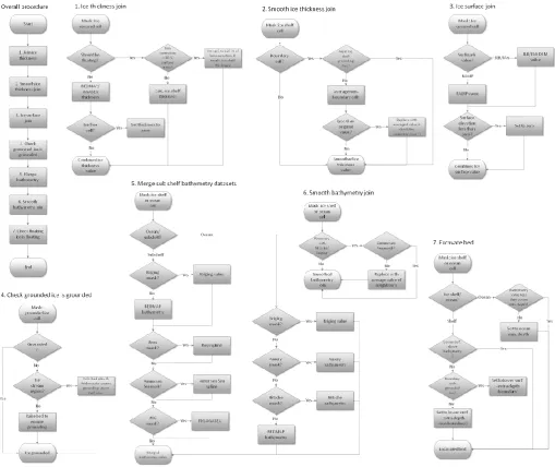
Figure 2 shows a flow diagram which works through the procedure carried out in this paper. The overall procedure consists of 7 steps which are documented further below. Firstly, the grounded and floating ice thickness datasets were joined, and the boundary smoothed to provide a smooth join.
Then a combined ice sheet surface DEM (Digital Elevation Model) was created, from two seperate DEMs. Next, the grounded ice sheet bed was derived from this surface and the combined thickness dataset. A check was then carried out to ensure that the ice is entirely grounded. All of the bathymetry datasets were then merged, the join smoothed in some regions, a flotation check was carried out, and areas where the ice is grounded were excavated.
3.1 Ice thickness
This section describes the merging of various sources of ice thickness data. Firstly, the merging of two grounded ice datasets is described (Sect. 3.1.1), then the merging of the grounded ice thickness with the floating ice shelf thickness (Sect. 3.1.2).
3.1.1 Grounded ice
Two versions of the ice thickness were produced, incorporat-ing different published datasets. The basic version includes the original BEDMAP ice thickness (Lythe et al., 2001) and the AGASEA/BBAS Amundsen Sea data (Vaughan et al., 2006; Holt et al., 2006). A second version was also produced, incorporating the Recovery Glacier region inferred ice thick-ness of Le Brocq et al. (2008) in addition to the BEDMAP and AGASEA/BBAS data. The ice thickness data is included in the netcdf dataset in the form of the lower ice sheet sur-face (lsrf and lsrf2) and topography (topg and topg2), derived from the ice thickness and ice surface topography. lsrf2 and topg2 refer to the second ice thickness version incorporat-ing the Recovery Glacier region modification. This section describes the method used to join the ice thickness datasets.
Firstly, the BEDMAP ice thickness was smoothed using a low pass filter (3×3 cell window), to remove spurious pat-terning present. It should be noted that the bed elevation dataset from BEDMAP is smooth in comparison to the ice thickness, so it is assumed that this was smoothed in the same way.
The region where there is dense coverage of RES (Radio Echo Sounding) flight lines in the AGASEA/BBAS dataset was identified, and the two datasets masked with a buffer zone where they overlap. The buffer zone has a width of 15 km. In the buffer zone, the two ice thickness grids were averaged and then smoothed to ensure a smooth join in the final dataset.
For lsrf2 and topg2, the Le Brocq et al. (2008) ice thick-ness was merged with the BEDMAP data in the same way as the AGASEA/BBAS dataset.
Figure 2.Flow diagram illustrating the processing procedure for the ice sheet configuration datasets.
Table 3.Summary of values used in the processing.
Description Value
Meteoric ice density (ρi) 918 kg m−3
Ocean density (ρw) 1028 kg m−3
Excavation extra depth (d) 20 m Excavation extra depth (next to grounding line, dgl) 1 m
3.1.2 Floating ice
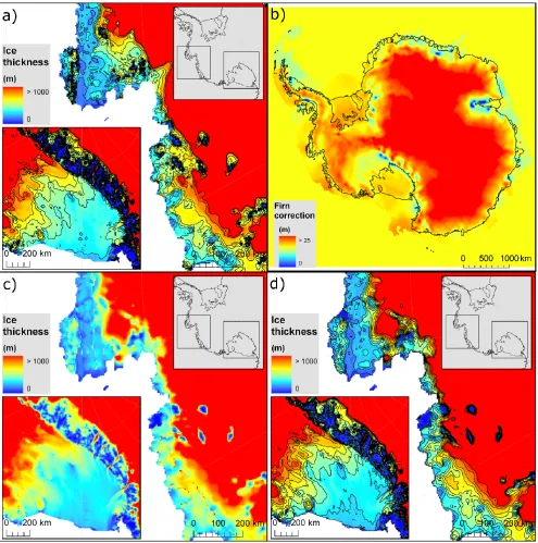
Many ice shelves around Antarctica do not have measure-ments of ice thickness available for them. The BEDMAP dataset used a hydrostatic assumption to derive ice shelf thickness from surface elevations measured from satellite al-timetry (see Fig. 3a for BEDMAP ice thickness). Since then, however, a new surface DEM has become available, incorpo-rating IceSat laser altimetry data, as well as radar altimetry (Bamber et al., 2009; Griggs and Bamber, 2009a). In order to calculate the ice shelf thickness from the surface elevation, the respective densities of ocean water and ice need to be specified and an estimate of the depth and density of the firn layer is also required. Since the BEDMAP dataset was com-piled, a spatial estimate of the firn correction for Antarctica has been produced using a regional climate model (RACMO, Van den Broeke et al., 2008, Fig. 3b). Therefore, the ice shelf thickness has been recalculated for the dataset presented in this paper.
The RACMO output (firn correction and accumulation) data were provided as lat-lon point measurements (equiva-lent resolution,∼55 km), these were reprojected onto the po-lar stereographic grid and interpolated onto the 5 km grid us-ing spline interpolation. Values away from the ice sheet in the original data are zero, these were ignored in the interpo-lation, leading to non-zero values over the grid. However, beyond the present day ice sheet, they have no basis, and are purely a function of the interpolation method. Therefore, the datasets were masked using the−2000 m bathymetry con-tour (to delimit the continental shelf) (Fig. 3b). Beyond the continental shelf, the mean value of the ice shelf firn values (16.5 m) is assigned.
Following Griggs and Bamber (2009b), the equivalent ice thickness (Hi, corresponding to the resulting ice thickness if
all the ice column was at the density of meteoric ice) is given by
Hi=
(s−f )ρw
ρw−ρi
, (1)
where s is elevation above sea level, f is a firn correction (defined as the difference between the actual depth of the firn layer and the depth that the firn would be if it was all at the density of meteoric ice),ρwis the density of sea
wa-ter,ρi is meteoric ice density. The actual ice thickness (H)
is, therefore, the equivalent ice thickness (Hi) plus the firn
correction ( f ),
H=Hi+f, (2)
and, hence,
H=(s−f )ρw ρw−ρi +
f. (3)
It is the actual ice thickness (H), i.e. meteoric ice thickness plus firn thickness, which is incorporated into the dataset
(i.e. usrf – lsrf, Fig. 3c). Any flotation calculation in an ice-sheet model should incorporate the firn correction in the cal-culation.
Equations (1) and (3) assume a constant density for ocean water (1028 kg m−3) and ice (918 kg m−3). In areas where surface melt occurs the firn correction is likely to be overesti-mated (Griggs and Bamber, 2009b; Michiel Van den Broeke, personal communication), however this is unlikely to affect the major ice shelves.
In some areas the firn correction is greater than the sur-face elevation, generally around the periphery of ice shelves where there is a high degree of uncertainty in the surface el-evation, or uncertainty as to whether shelf ice exists. Where the firn correction is greater than 80% of the surface eleva-tion, the surface elevation is set to 125% (100/0.8) of the firn correction value, and the ice shelf thickness calculated from this surface. These areas are indicated in umask (value of 4).
3.1.3 Joining ice thickness datasets
The grounded ice thickness and the ice shelf thickness must be joined smoothly to avoid any steep gradients in ice thick-ness. However, in order to maintain the consistency between the ice thickness and the ice surface in the ice shelf regions, the ice thickness cannot be smoothed in grounding line re-gions of the major ice streams. Hence, there is no smoothing carried out across the major ice stream grounding lines in the dataset presented here.
Away from the major ice stream grounding lines, the break in slope at the grounding line is more obvious and the surface DEM is less reliable due to “loss of lock” in the radar altime-try data (Griggs and Bamber, 2009a). This leads to a “con-tamination” of the surface heights in ice shelf regions close to the grounding line, and causes larger errors in the surface elevations and hence potentially elevated ice thicknesses. Ice thickness values in ice shelf cells that are on a border with the grounded ice were smoothed (average of “non-border” neighbours). The original value was then replaced with the smoothed value if the smoothed value was less than the orig-inal. This removes the spuriously high ice thickness values introduced at the grounding line by errors in the surface DEM (see Fig. 3d). A similar check to that in Sect. 3.1.2 was car-ried out to make sure that the smoothed ice thickness values were sufficient to lead to a surface elevation value greater than 125% of the firn correction.
3.2 Ice surface
Figure 3. Ice thickness join: (a) original BEDMAP ice thickness, (b) firn correction used in calculating the floating ice thickness, (c) unsmoothed combined grounded and floating ice thickness and (d) smoothed combined grounded and floating ice thickness. Contours show 100 m thickness intervals (up to 1000 m), they are not shown on (c) for clarity in showing the join between floating and grounded ice thickness datasets.
DEM (Antarctic Peninsula, Liu et al., 1999). The JLB/JAG DEM is derived solely from radar and laser altimetry, hence, the coverage is sparse over the Antarctic Peninsula and the DEM does not look realistic (Fig. 4a). The RAMP DEM in-corporates ADD elevation data over the Antarctic Peninsula, and whilst this also has large inherent errors, it is probably more accurate than the JLB/JAG DEM. The two were
Figure 4.Ice surface join: (a) hillshade of JLB/JAG DEM and (b) hillshade of combined DEM.
At this stage, the ice surface DEM is used, in combina-tion with the ice thickness, to calculate the bed elevacombina-tion in grounded areas of the ice sheet. Later, the surface elevation is re-calculated for ice shelf regions, and will differ from the original DEM, due to the ice thickness smoothing that oc-curred in Sect. 3.1.3. Small areas of the ice surface DEM, in grounded regions, are artificially raised in the next section, however these are not in ice stream regions, and generally are in areas where the DEM error is high.
3.3 Grounded ice covered bed
The bed elevation in the grounded ice region was derived by subtracting the grounded ice thickness (Sect. 3.1.1) from the combined ice surface dataset (Sect. 3.2). The ice thickness above buoyancy (H∗) was calculated using
H∗=(H−f )+(ρw/ρi)h, (4)
where h is bed elevation, and checked to ensure that the ice is grounded (where H∗≥0). There are two different areas where this may not be the case and these are treated sepa-rately:
1. where the ice surface/thickness is not confidently known, and away from major ice stream grounding lines. In these areas the bed elevation is increased to ensure the ice is grounded, hence the ice surface eleva-tion is altered. These areas are indicated with a value of 4 in umask, there are 544 grid cells which are altered, around 0.1% of the grounded ice cells.
2. ice stream areas, where it is important to keep the ice surface elevation the same as the DEM. In these regions the bed elevation and thickness needed to cause ground-ing, is calculated by rearranging Eq. (4) in terms of the
actual ice thickness (H) and surface elevation (s), where the surface elevation is taken from the surface DEM:
H=H
∗+f−(ρ
w/ρi)s
1−(ρw/ρi)
, (5)
where H∗here is set to 1 m.
The bed elevation (h) is then derived from
h=s−H. (6)
Ice free areas (see mask+) were checked to ensure that the bed elevation is above sea level, and their elevation set to a given elevation (10 m) if not.
3.4 Sub ice-shelf bathymetry
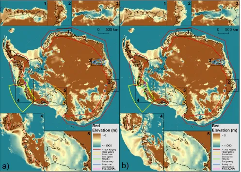
Away from the main ice shelves (e.g. Ross, Filchner-Ronne), there is very limited data on the sub ice-shelf bathymetry in BEDMAP. The interpolation algorithms employed by BEDMAP led to sub ice-shelf bathymetry values that caused many ice shelves to ground. This section describes the methods used to reinterpolate various areas of sub ice-shelf bathymetry. It should be emphasised here that the BEDMAP gridded datsets have been used for the reinterpolation, rather than the original BEDMAP database of measurements. The most straightforward method to ensure the ice shelves float would be to simply excavate a certain depth beneath the lower surface of the ice shelf, however this would lead to a uniform cavity depth, and this would not be realistic. The approach taken here is to carry out a slightly “supervised” ap-proach to the reinterpolation, identifying the problem areas, and tailoring the interpolation methods to each area. The bathymetry still requires excavation in certain areas, this is described in Sect. 3.4.6. The following sections describe the interpolation procedures for different areas: small ice shelves around East Antarctica (Sect. 3.4.1), the Ross Ice Shelf near the Transantarctic Mountains (Sect. 3.4.2), the Amundsen Sea region (Sect. 3.4.3), PIG (Pine Island Glacier) sub ice-shelf (Sect. 3.4.4) and the Amery sub ice-shelf region (Sect. 3.4.5).
It should be noted that the original BEDMAP bathymetry was on a slightly different coordinate reference than the BEDMAP ice thickness. When comparing the bathymetry with other datasets, it also appeared to be slightly offset. As a result, the BEDMAP bathymetry was shifted by−3134 m in the x-direction and 1866 m in the y-direction to remove this apparent shift and set the bathymetry grid’s spatial refer-ence to be the same as the ice thickness grid.
3.4.1 General (sub ice-shelf) bathymetry
Figure 5. Bed/bathymetry, coloured lines indicate masks where data was replaced: (a) original BEDMAP bed and bathymetry and (b) improved dataset. Insets show regions of interest described in the text: 1) and 2) General bathymetry, 3) Amery ice shelf, 4) Amundsen Sea region and 5) Ross Ice Shelf.
the mask overlies the major ice shelves (Ross/ Filchner-Ronne/Amery), as these are better constrained by observa-tion, or for ice shelves in the Amundsen Sea region, which are reinterpolated using a different method (see Sect. 3.4.3).
All ice shelf areas within the red outline shown in Fig. 5 were set to nodata, also, where the ocean bathymetry ele-vations were higher than−300 m, the elevation was set to nodata. The nodata values were then reinterpolated (using both grounded bed and bathymetry<−300 m) using kriging to produce deeper bathymetry (see Fig. 5).
3.4.2 Ross Ice Shelf
Near the Tranantarctic mountains, beneath the western Ross Ice Shelf, there are very few data available on the bathymetry. As a result, in combination with the Inverse Distance Weight-ing (IDW) interpolation used in BEDMAP, there is some “leakage” of the high elevations into the sub ice-shelf re-gion. This can be avoided by using a spline interpolation
technique, which would take into account the steep slope of the mountains towards the sub ice-shelf region, into the deep sub ice-shelf bathymetry. The most erroneous area was iden-tified by eye (see orange outline in Fig. 5). The area was then reinterpolated using a tension spline with a high weighting and high number of points in order to force the sub ice-shelf region near to the mountains to have a steep elevation gradi-ent, which levels offinto a deep, lower gradient surface away from the mountains (Fig. 5, inset 5).
3.4.3 Amundsen Sea Ice Shelves
data were combined with the grounded ice sheet bed from Sect. 3.3 and the BEDMAP bathymetry beyond the Nitsche dataset. The sub ice-shelf regions were then reinterpolated using a novel approach which allows the incorporation of the bathymetry data away from the ice shelf fronts.
The Nitsche et al. (2007) bathymetry suggests that the sub ice-shelf bathymetry is reasonably deep, with “trough” like features in the sub ice-shelf regions. As with the Ross Ice Shelf bathymetry (Sect. 3.4.2), this morphology lends itself to spline interpolation. However, away from the areas with ocean bathymetry data, even spline interpolation may lead to too shallow sub ice-shelf bathymetry and cause the ice shelves to ground.
Therefore, in order to aid the interpolation process, the “bottoms” of the troughs were imposed as a function of the ocean bathymetry at one end of a transect, and the grounded ice bed elevation at the other. A series of transects were con-structed (see red lines on Fig. 5, inset 4) and the sub ice-shelf bathymetry value, along the transect, calculated as a linear function of distance from either the ocean end of the tran-sect, or the grounded ice sheet end. Where two transects join, as beneath the Getz ice shelf, the transect connected to both the ocean and grounded bed is interpolated first, then the connecting transect uses the newly interpolated value at its connected end. These values were then combined with the masked bed/bathymetry data outside of ice shelf areas, and a spline interpolation carried out. The result is very diff er-ent from BEDMAP, and leads to deep sub ice-shelf cavities around the Amundsen Sea.
3.4.4 PIG Ice Shelf
Part of the PIG sub ice-shelf is treated differently to the rest of the Amundsen Sea ice shelves. Directly in front of PIG itself there is a trench connecting the ocean with the base of the ice stream. Rather than simply linearly interpolating the trench as in Sect. 3.4.3, the original AGASEA/BBAS data are used solely in the “trench”. Subsequent to this processing, a sub ice-shelf ridge has been identified (Jenkins et al., 2009).
3.4.5 Amery Ice Shelf
Whilst there are some data available for the sub ice-shelf bathymetry in the Amery Ice Shelf region in BEDMAP, there is also a large amount derived from interpolation, leading to a “ridge” appearing towards the coastal end of the ice shelf. Recent data suggests that this ridge does not exist (Galton-Fenzi et al., 2008), hence some reinterpolation has been carried out in the dataset presented in this paper. All bathymetry (sub ice-shelf and ocean) in BEDMAP that was above−600 m was reinterpolated using kriging, and replaced in the masked area shown on Fig. 5 (blue outline, also in-set 3), chosen to ensure a smooth join between the other datasets.
3.4.6 Excavation
In order to ensure that all the ice shelf regions will be floating, the bed was excavated in areas where the lower ice surface was below the bathymetry elevation (and the extra depth, see below) using
h=s−H−d, (7)
(where s has been recalculated using the smoothed ice thick-ness (using Eq. 3)), for cells not in proximity to grounded ice, where d is the extra depth specified beneath the ice shelf (20 m, see Table 3) and
h=s−H−dgl, (8)
for cells with a boundary with grounded ice, where dgl is
extra depth specified beneath the ice shelf next to grounding lines (1 m, see Table 3).
3.5 Ocean bathymetry
The ocean bathymetry (excluding sub-ice shelf areas) is largely the same as BEDMAP except in two areas, the Amundsen Sea and continental shelf areas as described in Sect. 3.4.1. This section describes the processing carried out in these regions.
3.5.1 Nitsche bathymetry
The BEDMAP bathymetry contains very few data from ob-servations in the Amundsen Sea region. The bathymetry dataset of Nitsche et al. (2007) is based on recent ship-based observations and provides a great improvement in the Amundsen Sea region. The published lat-lon data were re-projected onto the polar stereographic grid and interpolated onto the 5 km grid (see Fig. 5 for the result).
3.5.2 General (ocean) bathymetry
There are many ocean regions bordering ice shelves (partic-ularly in East Antarctia) which have elevations close to sea level (see Fig. 5, insets 1 and 2). This is not appropriate, as, if the ice shelves were to advance they would simply ground on these shallow regions and would not therefore flow in a realistic manner. There are very few data for the ocean bathymetry in these regions, hence, it is reasonable to carry out the same interpolation procedure as in the sub ice-shelf section (Sect. 3.4.1).
3.5.3 Final checks
Table 4.Summary of bmask values.
Value Description 0 BEDMAP
1 General bathymetry, areas>−300 m – reinterpolated (kriging) 2 Ross Ice shelf – Transantarctic Mountains – reinterpolated (spline)
3 Amundsen Sea ice shelves – small ice shelves reinterpolated (spline, with max depth derived from bathymetry) 4 PIG AGASEA/BBAS
5 Nitsche bathymetry 6 Amery Ice Shelf (kriging) 7 Smoothed join
8 Excavated bed – original bathymetry minus depth to make it float minus extra depth (20 m) 9 AGASEA/BBAS bed
10 BEDMAP/AGASEA join
11 Combined surface minus combined ice thickness
12 Bed elevation changed, ice thickness unchanged, surface not consistent with JLB/JAG 13 Bed and ice thickness changed, surface is consistent with JLB/JAG
14 Ocean>−10 set to−10
15 Excavated bed – original bathymetry minus depth to make it float minus extra depth (1 m)
Table 5.Summary of umask values.
Value Description 0 Ocean 1 Ramp surface
2 JLB/JAG surface grounded 3 JLB/JAG surface floating
4 Ice shelf areas not consistent with JLB/JAG surface (firn correction greater than surface) 5 Ice shelf thickness join smoothed and replaced if less than original
6 Shelf thickness changed because less resulting surface less than firn correction (post smoothing) 7 Missing/negative grounded ice thickness smoothed
8 Missing/negative grounded ice thickness replaced with 50 m 9 Ice free areas, ice thickness set to zero
10 Non-grounded ice: bed elevation changed, ice thickness unchanged, surface not consistent with JLB/JAG 11 Non-grounded ice: bed & ice thickness changed, surface is consistent with JLB/JAG
3.6 Summary of configuration datasets
The grids bmask and umask summarise the processing which has been carried out on the bed/bathymetry and ice sur-face/thickness configuration datasets respectively. Tables 4 and 5 detail the values provided in these masks.
Figure 6 shows the ice thickness above buoyancy for the original BEDMAP ice sheet configuration (Fig. 6a) and for the new dataset (Fig. 6b). The new dataset provides a much more consistent agreement with the grounding line suggested by the MOA dataset than BEDMAP.
4 Surface temperature
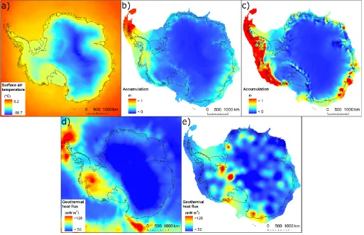
The surface air temperature dataset is described in Comiso (2000). The surface temperature estimates are derived from
AVHRR infrared data. Annual mean temperatures from 1982–2004 were averaged to provide the surface air temper-ature field (Fig. 7a). The AVHRR data is currently available on a monthly basis at a resolution of 6.25 km from Novem-ber 1978 to mid-2009 as part of an ongoing project.
5 Accumulation
5.1 Arthern et al. (2006)
Figure 6.Ice thickness above buoyancy: (a) original BEDMAP dataset and (b) ALBMAP dataset.
Figure 7.Other datasets provided: (a) surface air temperature, (b) accumulation (Arthern et al., 2006), (c) accumulation (Van de Berg et al.,
interpolated onto the 5 km grid using spline interpolation. In the original dataset there is no data beyond the ice sheet, however, it would be useful to have values beyond the present day ice sheet. Hence, the accumulation data was extrapolated beyond the present day ice sheet, though these values have no physical basis, and are purely the result of extrapolation from the ice covered values, and the interpolation method used, so should be used with caution. The accumulation dataset was masked using the−2000 m bathymetry contour (to provide data beyond the present day ice sheet, but to limit it to the continental shelf) (Fig. 7b).
5.2 Van de Berg et al. (2006)
The accumulation dataset of Van de Berg et al. (2006) is an output from the RACMO regional model (Van de Berg et al., 2006). The accumulation is generally higher than that of Arthern et al. (2006), especially in data-sparse areas. The integrated accumulation exceeds previous estimates by up to 15%. The data were provided as lat-lon point measure-ments, these were reprojected onto the polar stereographic grid and interpolated onto the 5 km grid using spline in-terpolation (Fig. 7c). The dataset was masked using the
−2000 m bathymetry contour in the same way as the Arthern et al. (2006) accumulation, again, areas beyond the present day ice sheet are a result of the extrapolation process and the interpolation method used.
6 Geothermal heat flux
Two geothermal heat flux maps are provided in this dataset, that differ greatly from each other. The method of deriva-tion is briefly described here and also the method of gridding the data. Note that the heat flux values are positive, some ice sheet models (including Glimmer-CISM), require these values to be negative.
6.1 Shapiro and Ritzwoller (2004)
Shapiro and Ritzwoller (2004) use a global seismic model of the crust and upper mantle to extrapolate existing heat flux measurements to areas where there are few data, using a “structural similarity function”. The original data are grid-ded on a geographic (lat-lon) grid, so when they are projected to a polar stereographic projection, this creates problems in gridding straight to 5 km resolution, due to the directionality of the points used in the interpolation procedure. The grid-ding introduces elongated features which are not present in the original data.
The effective resolution of the data (in latitude anyway) is∼100 km. Therefore the data were first gridded on to a 100 km grid using spline interpolation. The 100 km grid points were then reinterpolated, again using spline interpo-lation, onto the 5 km grid (Fig. 7d). This reduces the
elon-gated features whilst retaining most of the detail in the origi-nal dataset.
6.2 Fox Maule et al. (2005)
The geothermal heat flux dataset of Fox Maule et al. (2005) was derived from satellite magnetic data and a thermal model. The point data provided were interpolated on to the 5 km grid using spline interpolation. The dataset was then masked using the −2000 m bathymetry contour buffer de-scribed in Sect. 5, as the points are limited to the grounded ice regions of Antarctica (Fig. 7e).
7 Summary
This document has detailed the steps taken in order to cre-ate a dataset suitable for high resolution numerical ice sheet modelling. It is hoped that not only will the dataset be useful to the ice sheet modelling community, but also that the need for consistency within the ice sheet configuration datasets has been demonstrated. The importance of a consistent ice sheet surface across the grounding line cannot be empha-sised strongly enough, as well as the importance of a correct grounding line location. If a model is to accurately predict the future evolution of the ice sheet/ice streams it is important that the response is not just the model responding to inaccu-racies in the input data. Whilst these will never be eradicated, it is important that they are minimised as far as possible.
Acknowledgements. Thanks to those that have made their data
available directly or indirectly for this project, and given as-sistance in the construction of this dataset. It is impossi-ble to name all the contributors here, however Jennifer Griggs, Robert Arthern, Jonathan Bamber, Josefino Comiso, Laura Ed-wards, Cathrine Fox Maule, Frank Nitsche, Nicholai Shapiro, Ralph Timmerman, Michiel Van den Broeke, David Vaughan and Pippa Whitehouse have made specific contributions to the data and this manuscript.
Anne Le Brocq acknowledges funding from a UK Natural Environment Research Council (NERC) grant NE/E006108/1. Antony Payne acknowledges the support of the National Centre for Earth Observation. The work was also greatly helped by collabo-ration within the framework of the EU Framework 7 project ice2sea.
Edited by: O. Eisen
References
Arthern, R. J., Winebrenner, D. P., and Vaughan, D. G.: Antarc-tic snow accumulation mapped using polarization of 4.3-cm wavelength microwave emission, J. Geophys. Res.-Atmos., 111, D06107, doi:10.1029/2004JD005667, 2006.
Comiso, J. C.: Variability and trends in Antarctic surface tempera-tures from in situ and satellite infrared measurements, J. Climate, 13(10), 1674–1696, 2000.
Edwards, L. A.: Satellite Interferometry and Tracking data: Antarc-tic Velocity Map Generation, Validation and Application, Un-published PhD thesis, University of Bristol, UK, 2008.
Fox Maule, C., Purucker, M., Olsen, N., and Mosegaard, K.: Heat flux anomalies in Antarctica revealed by satellite magnetic data, Science, 309, 464–467, 2005.
Galton-Fenzi, B. K., Maraldi, C., Coleman, R., and Hunter, J.: The cavity under the Amery Ice Shelf, East Antarctica, J. Glaciol., 54(188), 881–887, 2008.
Griggs, J. A. and Bamber, J. L.: A new 1 km digital elevation model of Antarctica derived from combined radar and laser data – Part 2: Validation and error estimates, The Cryosphere, 3, 113–123, doi:10.5194/tc-3-113-2009, 2009a.
Griggs, J. A. and Bamber, J. L.: Ice shelf thickness over Larsen C, Antarctica, derived from satellite altimetry, Geophys. Res. Lett., 36, L19501, doi:10.1029/2009GL039527, 2009b.
Haran, T., Bohlander, J., Scambos, T., Painter, T., and Fahnestock, M. (compilers): MODIS mosaic of Antarctica (MOA) image map, Boulder, Colorado, USA, National Snow and Ice Data Cen-ter, Digital media, 2005 (updated 2006).
Holt, J. W., Blankenship, D. D., Morse, D. L., Young, D. A., Peters, M. E., Kempf, S. D., Richter, T. G., Vaughan, D. G., and Corr, H. F. J.: New boundary conditions for the West Antarctic Ice Sheet: Subglacial topography of the Thwaites and Smith glacier catchments, Geophys. Res. Lett., 33, L09502, doi:10.1029/2005GL025561, 2006.
Hubbard, A., Bradwell, T., Golledge, N., Hall, A., Patton, H., Sug-den, D., Cooper, R., and Stoker, M.: Dynamic cycles, ice streams and their impact on the extent, chronology and deglaciation of the British-Irish ice sheet, Quaternary Sci. Rev., 28(7–8), 758–776, 2009.
Jenkins, A., Dutrieux, P., Mcphail, S., Perrett, J., Webb, A., White, D., and Jacobs, S. S.: Bathymetry and ocean properties beneath Pine Island Glacier revealed by Autosub3 and implications for recent ice stream evolution, Eos Trans. AGU, 90(52), Fall Meet. Suppl., Abstract C31F-03, 2009.
Le Brocq, A. M., Hubbard, A., Bentley, M. J., and Bam-ber, J. L.: Subglacial topography inferred from ice surface terrain analysis reveals a large un-surveyed basin below sea level in East Antarctica, Geophys. Res. Lett., 34, L16503, doi:10.1029/2008GL034728, 2008.
Liu, H., Jezek, K., and Li, B.: Development of an Antarctic digital elevation model by integrating cartographic and remotely sensed data: A geographic information system based approach, J. Geo-phys. Res., 104(B10), 23199–23213, 1999.
Lythe, M. B., Vaughan, D. G.. and the BEDMAP Consortium: BEDMAP: A new ice thickness and subglacial topographic model of Antarctica, J. Geophys. Res.-Sol. Ea., 106(B6), 11335– 11351, 2001.
Meehl, G. A., Stocker, T. F., Collins, W. D., Friedlingstein, P., Gaye, A. T., Gregory, J. M., Kitoh, A., Knutti, R., Murphy, J. M., Noda, A., Raper, S. C. B., Watterson, I. G., Weaver, A. J., and Zhao, Z.-C.: Global Climate Projections, in: Climate Change 2007: The Physical Science Basis, Contribution of Working Group I to the Fourth Assessment Report of the Intergovernmental Panel on Climate Change, edited by: Solomon, S., Qin, D., Manning, M., Chen, Z., Marquis, M., Averyt, K. B., Tignor, M., and Miller, H. L., Cambridge University Press, Cambridge, UK and New York, NY, USA, 2007.
Nitsche, F.O., Jacobs, S., Larter, R. D., and Gohl, K.: Bathymetry of the Amundsen Sea continental shelf: Implications for geol-ogy, oceanography, and glaciolgeol-ogy, Geochem. Geophy. Geosy., 8, Q10009, doi:10.1029/2007GC001694, 2007.
Pattyn, F.: Transient glacier response with a higher-order numerical ice-flow model, J. Glaciol., 48(162), 467–477, 2002.
Pollard, D. and DeConto, R. M.: Modelling West Antarctic ice sheet growth and collapse through the past five million years, Nature, 458(7236), 329–333, 2009.
Price, S. F., Waddington, E. D., and Conway, H.: A full-stress, ther-momechanical flowband model using the finite volume method, J. Geophys. Res., 112, F03020, doi:10.1029/2006JF000724, 2007.
Scambos, T. A., Haran, T. M., Fahnestock, M. A., Painter, T. H., and Bohlander, J.: MODIS-based Mosaic of Antarctica (MOA) data sets: Continent-wide surface morphology and snow grain size, Remote Sens. Environ., 111(2–3), 242–257, 2007. Schoof, C.: Ice sheet grounding line dynamics: Steady states,
stability, and hysteresis, J. Geophys. Res., 112(F3), F03S28, doi:10.1029/2006JF000664, 2007.
Shapiro, N. M. and Ritzwoller, M. H.: Inferring surface heat flux distributions guided by a global seismic model: particular appli-cation to Antarctica, Earth Planet. Sc. Lett., 223, 213–224, 2004. Van de Berg, W. J., van den Broeke, M. R., and van Meijgaard, E.: Reassessment of the Antarctic surface mass balance using cali-brated output of a regional atmospheric climate model, J. Geo-phys. Res., 111, D11104, doi:10.1029/2005JD006495, 2006. Van den Broeke, M. R., van de Berg, W. J., and van Meijgaard, E.:
Firn depth correction along the Antarctic grounding line, Antarct. Sci., 20(5), 513–517, doi:10.1017/S095410200800148X, 2008. Vaughan, D. G., Corr, H. F. J., Ferraccioli, F., Frearson, N., O’Hare,