https://doi.org/10.5194/amt-12-6505-2019 © Author(s) 2019. This work is distributed under the Creative Commons Attribution 4.0 License.
Above-cloud aerosol radiative effects based on ORACLES 2016 and
ORACLES 2017 aircraft experiments
Sabrina P. Cochrane1,2, K. Sebastian Schmidt1,2, Hong Chen1,2, Peter Pilewskie1,2, Scott Kittelman1, Jens Redemann3, Samuel LeBlanc4,5, Kristina Pistone4,5, Meloë Kacenelenbogen5, Michal Segal Rozenhaimer4,5,6, Yohei Shinozuka5,7, Connor Flynn8, Steven Platnick9, Kerry Meyer9, Rich Ferrare10, Sharon Burton10, Chris Hostetler10,
Steven Howell11, Steffen Freitag11, Amie Dobracki12, and Sarah Doherty13
1Department of Atmospheric and Oceanic Sciences, University of Colorado, Boulder, CO 80303, USA 2Laboratory for Atmospheric and Space Physics, University of Colorado, Boulder, CO 80303, USA 3School of Meteorology, University of Oklahoma, Norman, OK 73019, USA
4Bay Area Environmental Research Institute, Mountain View, CA 94035, USA 5NASA Ames Research Center, Mountain View, CA 94035, USA
6Department of Geophysics and Planetary Sciences, Porter School of the Environment and Earth Sciences,
Tel-Aviv University, Tel-Aviv, Israel
7Universities Space Research Association, Mountain View, CA 94035, USA 8Pacific Northwest National Laboratory, Richland, WA 99354, USA 9NASA Goddard Space Flight Center, Greenbelt, MD 20771, USA 10NASA Langley Research Center, Hampton, VA 23666, USA
11Department of Oceanography, University of Hawaii, Honolulu, HI 96844, USA
12Department of Atmospheric Science, Rosentiel School of Marine and Atmospheric Science,
University of Miami, Miami, FL 33146, USA
13Joint Institute for the Study of Atmosphere and Ocean, University of Washington, Seattle, WA 98195, USA
Correspondence:Sabrina P. Cochrane ([email protected]) Received: 28 March 2019 – Discussion started: 26 April 2019
Revised: 16 August 2019 – Accepted: 16 October 2019 – Published: 9 December 2019
Abstract. Determining the direct aerosol radiative effect (DARE) of absorbing aerosols above clouds from satellite observations alone is a challenging task, in part because the radiative signal of the aerosol layer is not easily un-tangled from that of the clouds below. In this study, we use aircraft measurements from the NASA ObseRvations of CLouds above Aerosols and their intEractionS (ORACLES) project in the southeastern Atlantic to derive it with as few assumptions as possible. This is accomplished by using spec-tral irradiance measurements (Solar Specspec-tral Flux Radiome-ter, SSFR) and aerosol optical depth (AOD) retrievals (Spec-trometer for Sky-Scanning, Sun-Tracking Atmospheric Re-search, 4STAR) during vertical profiles (spirals) that mini-mize the albedo variability of the underlying cloud field – thus isolating aerosol radiative effects from those of the cloud field below. For two representative cases, we retrieve spectral
1 Introduction 1.1 Background
Aerosols are ubiquitous throughout the Earth’s atmosphere, and they play a crucial role in modulating the flux of solar ra-diation that reaches the Earth’s surface. The energy distribu-tion within a scene that contains aerosols depends not only on the amount of incoming solar radiation, aerosol optical depth (AOD), and type, but also on the albedo beneath the aerosols. Depending on the type of aerosol, the incoming radiation will be absorbed or scattered in a certain ratio, described by the single scattering albedo (SSA), while the direction (for-ward or back(for-ward) of the scattered radiation can be approx-imated by the asymmetry parameter (g). Aerosol absorption and scattering change the radiative balance relative to the aerosol-free atmosphere. This perturbation is called the direct aerosol radiative effect (DARE). The scene albedo below an aerosol layer, whether from clouds, ocean, or land, can de-termine whether the layer has a negative (positive) DARE, resulting in a cooling (warming) effect at the top of the at-mosphere (Twomey, 1977; Russell et al., 2002). Aerosols in-jected into the global climate system by human activity since the beginning of industrialization may offset up to 50 % of the warming due to anthropogenic greenhouse gas emissions (Myhre et al., 2013). However, the uncertainty of this off-set is large, in part due to observational challenges: radia-tive forcing by anthropogenic aerosol–radiation interactions could range from −1 to+0.2 W m−2(Fig. 8.15 in Myhre et al., 2013).
Deriving the direct effect of aerosols on the radiation bud-get, ignoring for the moment the impact on radiative balance due to aerosol influences on cloud properties and lifetime, is difficult since DARE is derived from the difference between radiative fluxes in the presence of and absence of aerosol. It is impossible to observe both states simultaneously, and there-fore, DARE is not directly measurable and, in most cases, requires a radiative transfer model (RTM) initialized with ob-servational or model inputs of aerosol AOD, SSA, andgas well as the spectral reflectance or albedo below the aerosol layer. The DARE calculations are limited by the accuracy of the observations and the model accuracy itself. For condi-tions where absorbing aerosols overlie inhomogeneous cloud fields, determining DARE is even more challenging since the calculations require both the aerosol properties as well as the cloud properties, primarily the cloud spectral albedo. The cloud radiative signal can be relatively large compared to that of aerosol particles. Therefore, it can be difficult to isolate the aerosol radiative effect from that of clouds, especially when the cloud albedo varies in the sampling region.
1.2 Satellite-derived cloud and aerosol properties to derive DARE
Obtaining the necessary cloud and aerosol parameters from satellite instruments provides the flexibility to estimate DARE in nearly any region. Until recently, aerosol and cloud properties could not typically be measured from the same satellite when the aerosol occurs above the clouds, and the strategy to estimate DARE for these conditions was to combine properties from multiple satellites (e.g., Chand et al., 2009; Meyer et al., 2013; Zhang et al., 2016; Sayer at al. 2016; Kacenelenbogen et al., 2019; Oikawa et al., 2018; Korras-Carraca et al., 2019). The problem with this approach, however, is that biases in the cloud and aerosol properties translate into biases in DARE if left unaccounted for (Meyer et al., 2013). For example, many DARE stud-ies utilize Moderate Resolution Imaging Spectroradiome-ter (MODIS) cloud optical thickness (COT) and effective droplet size (translated into cloud albedo, which cannot be directly measured from space) and/or AOD from the active lidar instrument Cloud-Aerosol Lidar with Orthogonal Po-larization (CALIOP). However, MODIS cloud retrievals can be biased when absorbing aerosols are present above cloud (Haywood et al., 2004; Wilcox et al., 2009; Coddington et al., 2010) and CALIOP AOD, which was known to be low-biased for daytime measurements (Kacenelenbogen et al., 2011; Winker et al., 2013; Meyer et al., 2013; Jethva et al., 2014) until the development of a new method in version 4 to derive AOD above cloud that uses the cloud returns to derive a much more accurate measure of AOD above cloud (Kim et al., 2018).
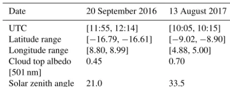
Table 1.Case description: spiral.
Date 20 September 2016 13 August 2017
UTC [11:55, 12:14] [10:05, 10:15]
Latitude range [−16.79,−16.61] [−9.02,−8.90] Longitude range [8.80, 8.99] [4.88, 5.00]
Cloud top albedo 0.45 0.70
[501 nm]
Solar zenith angle 21.0 33.5
value of SSA from the Southern African Regional Science Initiative (SAFARI) 2000 campaign to derive diurnal DARE. Jethva et al. (2013) estimate DARE using the SSA obtained from Aerosol Robotic Network (AERONET) sites. Since these measurements of SSA are not taken in conjunction with the other cloud and aerosol properties, it is difficult to deter-mine whether they are valid and consistent for the specific aerosol measured by the satellite.
Some studies, such as Peers et al. (2015) and de Graaf et al. (2012), have developed unique methods for which aerosol properties are not assumed. Peers et al. (2015) derive aerosol and cloud properties simultaneously through polarization measurements made by the Polarization and Directionality of Earth Reflectances (POLDER) instrument on the PARA-SOL satellite, while de Graaf et al. (2012) avoid the aerosol properties altogether and simulate a cloud-only sky and com-pare this to measured hyperspectral reflectances from the Scanning Imaging Absorption Spectrometer for Atmospheric Chartography (SCIAMACHY). de Graaf et al. (2019) com-pare DARE from these two methods along with DARE de-rived from OMI and MODIS for the southeastern Atlantic region, finding that DARE is correlated between all methods for moderate values of DARE. However, POLDER-derived values are higher than the other two methods for higher DARE values, which they attribute to larger cloud optical thickness retrievals by POLDER.
1.3 Estimates of DARE from aircraft observations Aircraft observations, as opposed to satellite remote sens-ing, provide in situ observations of clouds and aerosols that are better suited for deriving their radiative properties, espe-cially when the clouds are inhomogeneous. For example, an aircraft can fly through an aerosol layer to measure aerosol absorption, scattering, and SSA with in situ instruments or fly directly above a cloud layer to measure the albedo. Stud-ies such as Pilewskie et al. (2003), Redemann et al. (2006), Schmidt et al. (2010a), Coddington et al. (2010), LeBlanc et al. (2012), and Ehrlich et al. (2017) along with the work presented here have capitalized on this versatility and de-veloped new algorithms and instrumentation to determine aerosol and cloud properties, which can then be utilized to estimate DARE.
For example, under the specific conditions of an aerosol layer with a loading gradient above a homogenous, dark sur-face, Redemann et al. (2006) derived the below-layer aerosol forcing efficiency (radiative effect per mid-visible AOD) from the co-varying irradiance/AOD pairs along a leg with minimal dependence on radiative transfer calculations. This method, however, is not applicable for scenes with absorb-ing aerosols above clouds such as those encountered durabsorb-ing the recent NASA ObseRvations of CLouds above Aerosols and their intEractionS (ORACLES) project (Zuidema et al., 2016). The ORACLES project conducted three aircraft cam-paigns in the southeastern Atlantic, providing measurements in a region with high biomass burning aerosol loading where there have been few extensive field observations to date. In this study, we combine data from multiple instruments to re-trieve the aerosol and cloud properties as directly as possible in order to calculate DARE and investigate the relationship between DARE and cloud albedo. The sensitivity of DARE above the aerosol layer to the underlying surface can be de-scribed by the transition from a negative to a positive radia-tive effect, or cooling to warming (Russell et al., 2002). The albedo where this transition occurs, hereafter called the criti-cal albedo, expands upon the quantities of criticriti-cal reflectance and critical surface albedo that more specifically refer to the relationship between AOD and top of atmosphere reflectance (Fraser and Kaufman, 1985; Seidel and Popp, 2012). The de-pendence of the sign of the aerosol’s radiative effect on the underlying albedo has been shown for aerosols above clouds in the southeastern Atlantic by Keil and Haywood (2003), Chand et al. (2009), and Meyer et al. (2013).
ORACLES aircraft observations make up an extensive dataset that can be used to validate current satellite meth-ods of deriving the aerosol and cloud properties that go into calculations of DARE. To begin this process, our primary objective of this paper is to derive DARE as a function of (a) the aerosol optical properties and (b) cloud albedo from the ORACLES measurements. In Sect. 2, we describe the ob-servations themselves and the sampling approaches used to obtain them. Section 3 describes the methods used to deter-mine SSA andgand how we utilize the results to calculate DARE as directly as possible. Section 4 presents our find-ings, while Sect. 5 provides a discussion and ways in which we will explore DARE’s dependence on aerosol properties in the future, along with prospective satellite validation goals.
2 Observations: measurement techniques, instrumentation, and data
2.1 ORACLES
often covered by a seasonal stratocumulus cloud deck capped by a thick layer of biomass burning aerosols advected from the interior of the African continent, providing ideal natural conditions to assess aerosol radiative effects above various cloud scenes and improve the understanding of many aspects of cloud–aerosol interactions.
Both the NASA P-3 and the ER-2 aircraft were deployed in the 2016 campaign. The P-3 flew at approximately 5 km alti-tude and below, carrying a comprehensive payload of both in situ and remote sensing instruments. The ER-2 flew at high altitude, approximately 20 km, carrying remote sensing in-struments such as the enhanced MODIS Airborne Simulator (eMAS) and the High Spectral Resolution Lidar 2 (HSRL-2) that collected simultaneous and collocated measurements with the P-3 during several coordinated flights. During the 2016 deployment, the P-3 completed 14 science flights in total, 5 of which were collocated with the ER-2 and 9 of which included radiation-specific sampling maneuvers. Al-though the ER-2 did not participate in the 2017 deployment, the P-3 payload remained nearly the same except for the ad-dition of HSRL-2 that had been deployed on the ER-2 during the 2016 campaign. Therefore, we focus on utilizing mea-surements taken from the P-3, which conducted 12 science flights in total, with 5 flights dedicated to radiation-specific studies in 2017. In this study, we primarily use measure-ments taken by SSFR, 4STAR, and HSRL-2 to investigate two cases, 20 September 2016 and 13 August 2017, which met specific requirements such as varying scene albedos and large aerosol loading. A companion paper will present more generalized results.
2.2 SSFR and ALP
The SSFR (Pilewskie et al., 2003; Schmidt and Pilewskie, 2012) is comprised of two pairs of spectrometers. Each pair consists of one spectrometer that is sensitive over the near-ultraviolet, visible and very near-infrared wavelength range, and another that is sensitive in the shortwave infrared wave-length range. The spectra are joined at 940 nm to provide a full spectral range from 350 to 2100 nm. The SSFR mea-sures downward spectral irradiance (Fλ↓) from a zenith light collector mounted on a stabilizing platform on the upper fuselage and upward spectral irradiance (Fλ↑) from a nadir light collector fix-mounted to the aircraft. The externally mounted light collectors are connected by fiber optic cables to the spectrometer, which resides in the aircraft cabin along with the data acquisition unit. The SSFR was radiometrically calibrated with a NIST-traceable 1000 W lamp light source before and after each deployment, and relative calibration changes throughout the field campaign were monitored with a portable field standard. The light collectors consist of an in-tegrating sphere with a circular aperture on top. They weigh the incoming radiance according to an angular response close to the cosine of the incidence angle. These light collectors have been improved over time (Kindel, 2010) to minimize
the dependence on the azimuth angle of the incident radiance. However, the dependence on the polar angle, termed the co-sine response, still requires careful characterization in the laboratory before and after the deployment. After applying all corrections, the uncertainty of the SSFR measurements is 3 %–5 % across the spectral range for both zenith and nadir irradiance. More importantly for this study, the precision is 0.5 %–1.0 %.
The zenith light collector of SSFR was kept horizontally aligned by counteracting the variable aircraft attitude with an Active Leveling Platform (ALP), which was developed at CU Boulder for the NASA C-130 aircraft (Smith et al., 2017) and later rebuilt for the P-3, specifically for ORACLES. ALP re-lies on aircraft attitude information from a dedicated inertial navigation system (INS) that monitors the aircraft attitude, specifically the pitch and roll angles. This information is sent to a real-time controller, which additionally has the ability to instead ingest data from the aircraft INS. The controller drives the two actuators of a two-axis tip–tilt stage: one axis for aircraft roll movements and one for aircraft pitch move-ments. As the attitude angle changes, the tip–tilt stage adjusts accordingly to maintain the SSFR at the horizontal level po-sition within approximately 0.2◦. The nadir light collector was not actively leveled since the horizontal cloud variabil-ity introduces much more variabilvariabil-ity into the signal than any attitude changes. The upwelling irradiance is also less sensi-tive to pitch and roll angles than the downwelling irradiance. For fix-mounted zenith light collectors, not only will the downward irradiance be referenced to an incorrect zenith due to the polar angle of incident light referenced to the air-craft horizon rather than true horizontal, but radiation from the lower hemisphere will also contaminate the zenith ir-radiance measurements if the receiving plane is not prop-erly aligned with the horizon. This is especially problem-atic over bright surfaces such as snow, ice, or clouds. For ORACLES, it was important to sample the dependence of the downwelling irradiance on the aerosol conditions above. Since the aerosol-induced irradiance changes are small com-pared to the reflection by clouds, even minor contamination from the lower hemisphere could cause a bias in the signal. Such biases cannot be corrected in post-processing because common correction schemes assume that no radiation origi-nates in the lower hemisphere (Bucholtz et al., 2008). ALP alleviates these problems and enables the collection of irra-diance data during spiral measurements as long as pitch and roll stay within the ALP operating range of 6◦. For the rea-sons mentioned above, spiral data have traditionally not been useful for radiation science. In this study, they turn out to be the key for achieving our stated goals.
2.3 4STAR, HSRL-2, and eMAS
available in the main ORACLES data archive (ORACLES Science Team, 2017a, b, 2019). The instrument is calibrated before and after each deployment using the Langley plot technique (Schmid and Wehrli, 1995); in addition, correc-tions for non-uniform azimuthal dependence of the trans-mission of the optical fiber path were assessed after each flight calibration (Dunagan et al., 2013) and corrected for in post-processing, resulting in an average AOD uncertainty of 0.011 at 500 nm (LeBlanc et al., 2019). 4STAR also provides other quantities, for example, column water vapor and trace gas retrievals, which are not used here. HSRL-2 is a downward-pointing lidar that provides vertical profiles of aerosol backscatter and depolarization at 355, 532, and 1064 nm wavelengths. Aerosol extinction is measured at 355 and 532 nm wavelengths (Hair et al., 2008; Burton et al., 2018). When the ER-2 was collocated with the P-3; imagery from the eMAS multispectral imager (King et al., 1996; Ellis et al., 2011) provided scene context.
2.4 Methods of sampling: radiation walls and spirals There are two ways to determine aerosol-intensive opti-cal properties from irradiance and AOD. An algorithm by Schmidt et al. (2010a) uses nadir and zenith irradiance pairs above and below a layer to retrieve SSA,g, and the surface albedo. A different algorithm, by Bergstrom et al. (2010), first derives the layer absorption and scene albedo from the irradiance pairs above and below the layer and then infers SSA, assuming a fixed value for g. Both methods were ap-plied to clear sky and require irradiance measurements above and below a layer along with the associated AOD, which are most often obtained from individual points along the upper or lower leg of a “radiation wall” as shown in Fig. 1.
The intent of the wall is to obtain scene albedo, layer ab-sorption, or transmittance by bracketing the aerosol layer above and below when flying at multiple altitudes along a track of about 100 km length. When only one aircraft is avail-able, it samples the required legs sequentially, taking over an hour to complete. In clear sky, an aerosol layer will likely not change substantially during this time. However, in cloudy skies such as those encountered during ORACLES, the time lag between sequential sampling of the upper and lower legs is large enough that the cloud field is likely to change. Fig-ure 1 illustrates the sampling for only two altitudes: at the bottom of the layer (BOL) and at the top of the layer (TOL) of interest. In the case of ORACLES, the BOL leg is located just below the aerosol layer and just above the cloud layer, where the column AOD and scene albedo are measured. The TOL leg is above the aerosol layer and the cloud, from which HSRL-2 measures profiles of extinction. Many other legs, for example below and within the cloud, and within the aerosol layer, were typically flown in addition to the BOL and TOL legs.
The net irradiance (Fλnet) at any level is the difference be-tween the downwelling and upwelling irradiance. The
ab-Figure 1.Schematic of a radiation wall, radiation spiral, and the appearance of horizontal flux divergence (Hλ) in SSFR
measure-ments. During a radiation wall, SSFR measures upwelling and downwelling irradiance along the top of layer leg (TOL) and bottom of layer (BOL) leg, which are collocated in space but not in time. During the radiation spiral, SSFR measures upwelling and down-welling irradiance throughout the entire aerosol layer. The left-hand side of the figure illustrates an example of how non-zeroHλarises
in SSFR measurements under certain cloud conditions. The gray tri-angles figuratively represent the viewing geometry of SSFR at the TOL and BOL. Ignoring any change in clouds over time, the TOL SSFR-measured irradiances include contributions from a larger area than at the BOL. Under inhomogeneous conditions, the TOL and BOL SSFR measurements contain differing cloud scenes; in our il-lustration, the BOL measurement has little to no signal contribution from clouds, whereas the TOL measurement has a large contribu-tion of the signal from clouds. The upwelling irradiance at the TOL would therefore be larger (smaller net irradiance) than at the BOL (larger net irradiance) due to the bright clouds.
sorption Aλ of a layer can be determined from the
differ-ence of the net irradiance at the upper and lower bound-aries (the vertical componentVλ of the flux divergence) if
the horizontal flux divergence of radiationHλ is negligible
(|Hλ|< <|Vλ|). Under horizontally homogeneous conditions,
we assumeAλ=Vλ, which is usually the case, giving
Aλ=Vλ=
Fλ,nettol−Fλ,netbol Fλ,↓tol
= h
Fλ,↓tol−Fλ,↑tol−Fλ,↓bol−Fλ,↑boli Fλ,↓tol ,
(1a)
whereAλandVλhave been normalized by the incident
irra-diance at the top of the layer (Fλ,↓tol). Under partially cloudy conditions,
Aλ=Vλ−Hλ. (1b)
Schmidt et al. (2010b) found thatHλof a cloud layer is not
negligible and can attain a magnitude comparable toAλ
bracketing the cloud layer with irradiance measurements. For ORACLES, the aerosol above clouds, rather than the cloud itself, constitutes the layer of interest, but Fig. 1 illus-trates how non-zero values of Hλ may arise under
inhomo-geneous conditions. The aerosol retrievals are only accurate if|Hλ|< <|Vλ|, which ensures that Eq. (1a) holds. The data
analysis showed that this condition was rarely met for wall measurements, but more often during spiral measurements (Sect. 3.1).
The radiation spiral, shown in Fig. 2 and illustrated con-ceptually in Fig. 1, provides multiple irradiance and AOD samples throughout the layer. Such a sampling pattern pro-vides irradiance measurements at four headings throughout the column at a high vertical resolution without increasing the duration of the profile because the aircraft keeps descend-ing or ascenddescend-ing durdescend-ing the straight segments, typically at 1000 feet (approximately 305 m) per minute. During ORA-CLES, spirals were on average completed over the course of 10–20 min, depending on the vertical extent of the aerosol layer. Since typical roll angles during turns were 15–30◦, exceeding the operating range of ALP, the spirals include short, straight segments of 20–30 s duration every 90◦ head-ing change. The small pitch and roll values durhead-ing the straight segments can be corrected for in real time by the ALP and lead to a rounded square-shaped pattern as shown in Fig. 2b and d rather than a traditional, circular spiral pattern. SSFR acquires the irradiance profile over a minimal horizontal ex-tent approximately 10 km in both latitude and longitude, re-ducing cloud and aerosol inhomogeneity effects, and over a much shorter time interval relative to the wall, maintain-ing correlation of measured irradiances throughout the spiral to the ambient cloud field. A circular spiral pattern with no straight segments with a roll angle under the roll limit would cover too large an extent, and the benefits of the square spi-ral pattern would be lost. Moreover, the four heading angles allow biases from mechanical mounting offsets of ALP or reflections and obscuration by the aircraft structure to be di-agnosed. Acquiring a large number of samples over a rel-atively limited horizontal extent also reduces the impact of cloud albedo variability on the nadir irradiance. The down-side of the spiral sampling is that it does not capture the spatial variability of the scene albedo, which is assessed by the radiation wall. Therefore, in order to investigate any spa-tial relationships between radiative effects and albedo, spiral measurements must be used in conjunction with AOD and scene albedo measurements from the radiation wall where the albedo is defined as
albedoλ=
Fλ↑ Fλ↓
. (2)
2.5 Case selection
To characterize the connections between DARE, aerosol properties, and scene albedo, we chose to explore cases based
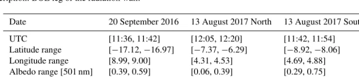
on (a) the availability of measurements from both a radiation wall and a radiation spiral, (b) relatively high aerosol load-ings above the cloud field, and (c) a range of measured albe-dos. The first case is 20 September 2016, where the spiral was located approximately 2.5 degrees of longitude off the coast near the Namibia/Angola border. The cloud field for this case was homogeneous; the albedo of the BOL leg of the radiation wall ranged from 0.39 to 0.59 at 501 nm. The radiation spiral was located at the northern end of the BOL leg. The aerosol layer was geometrically and optically thick, with an AOD measured just above clouds during the spiral of 0.57 at 501 nm. The ER-2 flew in coordination with the P-3, such that eMAS imagery is available for context. Figure 2b shows an eMAS image overlaid with the flight track of the P-3 for the spiral flight pattern, along with the ER-2 flight track. The second case on 13 August 2017, located approx-imately 8 degrees of longitude off of the coast of northern Angola, was chosen because of the inhomogeneous cloud conditions encountered along the BOL leg of the radiation wall. We treat this leg of the radiation wall as two separate cases based on differing albedo ranges – the northern end of the wall, where the albedo values at 501 nm range from 0.06 to 0.39, and the southern end of the wall, where the albedo at 501 nm ranges from 0.29 to 0.75. The radiation spiral was lo-cated on the southernmost point, though we use the retrieval results for both the North case and South case DARE calcula-tions. Fig. 2d shows the spiral flight path overlaid on visible imagery from SEVIRI (Spinning Enhanced Visible and In-frared Imager) onboard the geostationary Meteosat Second Generation (MSG) (Schmid, 2000). The aerosol layer was significantly thinner than that of 20 September 2016, with an AOD at 501 nm measured just above clouds during the spiral of 0.22. Table 1 lists the important parameter ranges for both spirals: UTC, latitude, longitude, solar zenith angle (SZA) and albedo at cloud top. Table 2 lists these parameters for the BOL legs for each of the three cases.
3 Methods
Figure 2.The(a)latitude vs. altitude and(b)longitude vs. altitude of altitude-filtered spiral data for 20 September 2016.(c)The corre-sponding high-resolution eMAS imagery (blue) with lower resolution MODIS imagery (gray). Overlaid is the P-3 spiral flight track in green and ER-2 flight track in red.(d)The latitude vs. altitude and(e)longitude vs. altitude of altitude-filtered spiral data for 13 August 2017. (f)Corresponding SEVIRI imagery. For 20 September 2016, the altitude range is 1.4 to 6.5 km, while for 13 August 2017 the altitude range is 1.7 to 5 km. For all four figures, the purple color shows data that are within the limits of the ALP but do not pass the geographic or standard deviation filter. The orange color shows the data that have passed the geographic filter but do not pass the standard deviation filter. The blue points meet all of the requirements and are the data used within the linear fit to determine the TOL and BOL irradiances.
Table 2.Case description: BOL leg of the radiation wall.
Date 20 September 2016 13 August 2017 North 13 August 2017 South
UTC [11:36, 11:42] [12:05, 12:20] [11:42, 11:54]
Latitude range [−17.12,−16.97] [−7.37,−6.29] [−8.92,−8.06]
Longitude range [8.99, 9.00] [4.31, 4.53] [4.69, 4.88]
Albedo range [501 nm] [0.39, 0.59] [0.06, 0.39] [0.29, 0.75] Solar zenith angle range [18.5, 18.8] [22.1, 22.3] [22.7, 23.5]
3.1 Irradiance measurements: walls vs. spirals
To derive accurate aerosol absorptance from SSFR measure-ments, irradiance pairs above and below the layer must first be obtained. For the radiation walls, the irradiance pairs are sampled from the BOL and TOL legs at coincident locations, neglecting cloud advection and cloud evolution during the elapsed time between the two. For spirals, the entire measure-ment profile from above cloud to above aerosol is used to es-tablish a linear fit of the data from which irradiance pairs are derived, improving the sampling statistics compared to
ra-diation wall irradiance pairs. Figure 3 illustrates SSFR mea-sured nadir and zenith irradiances for aircraft attitudes within the operating range of ALP plotted against the 4STAR AOD at 532 nm as a vertical coordinate. Uncertainty bars are in-cluded for a subset of the measurements. Prior to fitting, all data are corrected to the SZA at the midpoint of the spiral to account for the minor change in solar position throughout the spiral:
Fλ=Fλ×
µ0
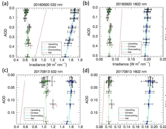
Figure 3.Examples of the filtering and extrapolation technique for 20 September 2016(a)532 nm and(b)1602 nm and for 13 August 2017 radiation spirals at(c)532 nm and(d)1602 nm. SSFR irradiance measurements are plotted against 4STAR above-aircraft AOD at 532 nm along with the associated measurement uncertainty. The omitted upwelling data (pink) did not pass the standard deviation or geographic filter and is not used for the calculation of the linear fit. All zenith measurements are included in the fit. At 1602 nm, there is little to no aerosol absorption and the net irradiance is expected to be nearly constant with altitude. At 532 nm however, there is aerosol absorption and the net irradiance decreases with increasing AOD.
whereµ=cos(SZA)andµ0is the value at the midpoint of
the spiral.
To derive the BOL and TOL irradiances from the spiral using all the data, a linear regression is performed:
Fλ↑=a↑λ+b↑λ×AOD532, (4a)
Fλ↓=a↓λ+b↓λ×AOD532, (4b)
whereaλ andbλ are the slope and intercept of the linear fit
lines. The data points from the spiral are used collectively to establish the fit coefficients in Eqs. (4a) and (4b), which express the change in nadir and zenith irradiance with AOD. Subsequently, the irradiance values at BOL and TOL are de-termined from AODmax532, measured at the bottom of the layer, and AODmin532, measured at the TOL. This method is more ro-bust than picking individual irradiance pairs from the wall because many more data points are used. The uncertainty of the fit coefficients is dominated by the variability of the data throughout the vertical profile, rather than by the radiometric uncertainty of the contributing data points, discussed in more detail in Sect. 3.4.
At a wavelength with small aerosol effects, such as 1.6 µm, shown in Fig. 3b, d, neither nadir nor zenith irradiance change significantly as the aircraft moves through the layer.
Any observed non-linearity or variability in the vertical pro-file at this wavelength can be ascribed to spurious measure-ment errors: for zenith, these could be due to reflections or obstructions by the aircraft or other factors causing a tran-sient variability in the downwelling irradiance. For nadir, this is attributed to albedo changes in the cloud field below. By contrast, the irradiance at 532 nm (Fig. 3a, c) changes con-siderably throughout the vertical profile. The zenith irradi-ance decreases with decreasing altitude due to the increasing attenuation by the aerosol layer. The nadir irradiance shows the opposite behavior, decreasing with increasing altitude. By comparison, zenith and nadir irradiance would change in lock step for a purely scattering layer because the net irradi-ance remains constant in the absence of absorption.
3.1.1 Data filtering
To ensure that the aerosol signal is isolated from that of the variability of the underlying scene and that the data quality is sufficient to produce reasonable retrievals of SSA andg, a series of data filtering steps are applied.
varia-tions due to horizontal changes in the cloud field un-derneath (nadir) or any variability in the zenith signal unrelated to the aerosol layer. Figure 2a, c show the spi-ral data as a function of altitude, with color coding to highlight data that passes the altitude filter.
2. Select a subset of nadir data to focus on either predom-inantly clear or cloudy regions within the geographical footprint of the spiral. For the 20 September 2016 spiral, we focused on the cloudy pixels by selecting a longitude range of 8.86 to 8.98◦E based on the eMAS imagery, illustrated in Fig. 2b, thereby eliminating regions that were substantially darker than the rest of the scene. The 13 August 2017 spiral did not require this filter because there were no clear regions distinguishable from cloudy regions (Fig. 2d).
3. Exclude data points where the nadir irradiance at 1.6 µm exceeds 1 standard deviation of the mean. These points are rejected to minimize the impact of cloud spatial in-homogeneity on the upwelling signal. Fig. 3 indicates for each case the points that are included in the zenith and nadir linear fits and those that are outside of the standard deviation limit. The data points that are outside of the altitude and geographic filters are not shown. The aerosol loading on 13 August 2017 was significantly lower than on 20 September 2016, as well as the num-ber of valid SSFR data points. This case was specifically chosen to explore the feasibility and sensitivity of the retrieval to variability in the upwelling irradiances and aerosol loading.
3.1.2 Horizontal flux divergence
Having obtained irradiance pairs from the wall or the spi-ral, the next step is to ensure that |Hλ| |Vλ| to
mini-mize the impact of horizontal flux divergence in the sub-sequent retrieval of aerosol-intensive optical properties. At long wavelengths,Hλ asymptotically approaches a constant
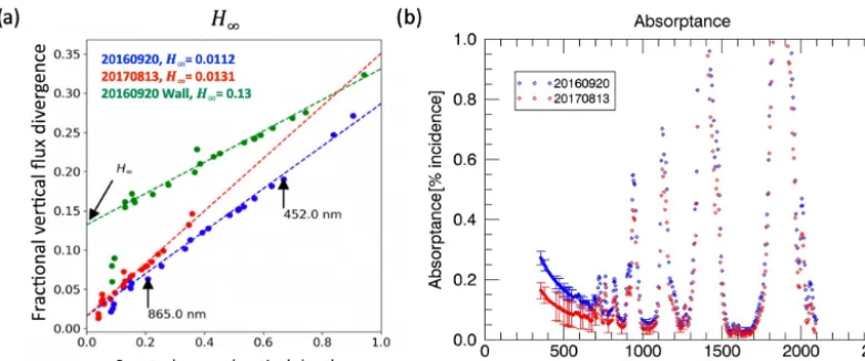
value as described by Song et al. (2016), which we denote asH∞. At the same time, aerosol absorption decreases with increasing wavelength (and thus decreasing optical thick-ness). Figure 4a shows Vλ plotted as a function of AODλ
for 20 September 2016 and 13 August 2017. The intercept at AOD=0 (A=0 by definition) determinesHλ because any
non-zero measurement ofVλ must originate fromHλ in the
absence of absorption. In the limit ofλ→ ∞,
limAOD(λ)→0Vλ≡H∞. (5)
Thus, even though we do not determineHλdirectly,H∞is straightforward to obtain. Because of the findings of Song et al. (2016),Hλ is zero for all wavelengths ifH∞ is zero. Therefore, it is justified to apply Eq. (1) to estimateAλonly
ifH∞=0.
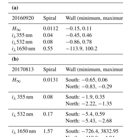
Table 3. (a)H∞and selectiλ values for the 20 September 2016
case.(b)H∞and selectiλvalues for the 13 August 2017 case.
(a)
20160920 Spiral Wall (minimum, maximum)
H∞ 0.0112 −0.15, 0.11 iλ355 nm 0.04 −0.45, 0.46
iλ532 nm 0.08 −0.86, 0.78
iλ1650 nm 0.55 −113.9, 100.2
(b)
20170813 Spiral Wall (minimum, maximum)
H∞ 0.0131 South:−0.65, 0.06 North:−0.83,−0.29
iλ355 nm 0.08 South:−1.9, 0.35
North:−2.22,−1.35
iλ532 nm 0.17 South:−5.4, 0.59
North:−5.43,−2.68
iλ1650 nm 1.57 South:−726.4, 3832.95
North:−410.8,−4.94
Table 3a and b show that the calculatedH∞ values for the filtered spiral data are near zero but significantly higher for the walls. For the 2016 case,H∞=1.12 % for the spiral and up to 15 % for the irradiance samples from the wall.H∞ is larger for the 13 August 2017 spiral, about 1.3 %, which could be due to the larger scene inhomogeneity based on the available imagery. It makes sense that the wall measure-ments have larger values forH∞, mainly because the col-located pairs do not necessarily represent the irradiance of the same scene, considering the time difference between the BOL and TOL legs. In addition, the effective footprint of the nadir SSFR light collector (the circle from within which half of the signal originates) changes at different altitudes, which means that the horizontal extent of cloud that contributes to the sampled signal for the TOL leg is much greater than for the BOL leg. While this is also true for the spiral, the stan-dard deviation filtering effectively separates the aerosol sig-nal from that of changes in scene albedo, including those due to the changing footprint size of SSFR with altitude.
To quantify the horizontal variability in the flux field rela-tive to the aerosol absorption, we introduce the inhomogene-ity ratio
iλ=
H∞ Vλ−H∞
. (6)
The denominator approximates the true absorption, where the horizontal flux contribution to the observedVλ has been
subtracted to yieldAλ (though we have substitutedH∞for Hλ).Vλ andH∞are both measurable quantities, whileAλ
Figure 4.Examples of the method for determiningH∞.Vλis shown as a function of AODλ for all 4STAR wavelengths for both cases
(20160920 in blue; 20170813 in red) along with an example point from the 20160920 radiation wall. At long wavelengths, the horizontal flux divergenceHλ asymptotes to a constant value(H∞); a non-zero value indicates 3-D effects. Here we perform a linear fit between
AODλ,maxandVλ, the vertical flux divergence, for all 4STAR wavelengths whereH∞is theyintercept, thereby bypassing the necessity of determiningHλdirectly. Figure 4b: the spiral derived for 20 September 2016 and 13 August 2017. Uncertainty estimates are shown as error
bars at the 4STAR wavelengths.
be of similar magnitude, and we cannot determineAλ from
Vλ. The spectral inhomogeneity metric provides an empirical
method to determine when this occurs.
Table 4 summarizes the interpretation ofiλ values, which
can be either positive or negative due to the horizontal flux divergence; when iλ is positive, this indicates a divergence
of radiation within the layer (apparent absorption), and when iλis negative it indicates a convergence (apparent emission).
We expect that as the wavelength becomes longer, the mag-nitude ofiλwill also increase since the aerosol absorption is
largest at the shortest wavelengths, whileHλis not strongly
wavelength dependent. Table 3a and b list the iλ values at
355, 532, and 1650 nm for the spiral and, for illustration, the maximum and minimumiλvalues from the radiation walls.
Both spirals exhibit near-zero iλ values at 355 and 532 nm,
though the 13 August 2017 values are slightly closer to 1, in large part due to the lower aerosol loading, and the re-trieval from 20 September 2016 is therefore more reliable than 13 August 2017. The maximum (minimum) iλ values
for the radiation walls are larger (smaller) than the spiral val-ues at all wavelengths. The specificiλvalues for which
per-forming an aerosol retrieval is minimally affected byHλare
subjective, and a follow-up paper will further develop and characterize the limits by investigating more cases from OR-ACLES.
Because of the highH∞andiλvalues, the wall
measure-ments are not used to determine aerosol absorptance or for the SSA andgderivation. Conversely, the near-zeroH∞ val-ues and low iλ values of the spirals allow us to substitute
Table 4.Interpretation ofiλrelating to the relative magnitudes of
VλHλ.
iλ ±1 < 1 >−1 > 1 <−1
Relative Vλ∼Hλ Vλ> Hλ Vλ< Hλ
Magnitude
Successful aerosol Unlikely Likely Not possible retrieval
Eqs. (4a) and (4b) into Eq. (1), which simplifies to
Aλ=
AODmax532 ×b↑λ−b↓λ aλ↓
. (7)
The spiral-derived absorptance spectra for (a) 20 Septem-ber 2016 and (b) 13 August 2017 are shown in Fig. 4b. The largest absorptance occurs in the water vapor bands of 1870, 1380, 1100, and 940 nm. In the relatively water-free spec-tral range, approximately 900 nm and shorter, the absorp-tance is dominated by aerosol absorption (except for a few water vapor bands with relatively low absorption, the oxy-gen A- and B-bands, the Chappuis ozone absorption band, and other trace gas absorption). The 4STAR AOD retrieval wavelengths specifically avoid the gas absorption features, although those that coincide with the Chappuis ozone ab-sorption band and other trace gas abab-sorption bands are un-avoidable and are accounted for in the 4STAR retrieval (see the Appendix of LeBlanc et al., 2019).
we assume that sinceAλis unaffected by cloud
inhomogene-ity whenH∞is near zero, the same is true for the irradiances from whichVλ is originally calculated.H∞andiλ serve as
metrics to assess the suitability of data for the aerosol re-trieval.
3.2 SSA retrieval
The retrieval of SSA and gis done with publicly available one-dimensional (1-D) radiative transfer model (RTM) DIS-ORT 2.0 (Stamnes et al., 2000), with SBDART for atmo-spheric molecular absorption (Ricchiazzi et al., 1998) along with the standard tropical atmosphere available within the libRadtran public library (Emde et al., 2016; http://www. libradtran.org, last access: 15 November 2019). In contrast to the algorithms by Pilewskie et al. (2003), Bergstrom et al. (2007), and Schmidt et al. (2010a), the aerosol layer is lo-cated over a variable cloud scene, but otherwise the principle is the same. This work is most similar to the algorithm intro-duced by Schmidt et al. (2010a), for which SSA andg are retrieved simultaneously.
The RTM allows us to calculate upwelling and down-welling fluxes determined by inputs of the surface albedo and the aerosol properties of AOD, SSA, and the asymme-try parameter. The updated retrieval algorithm is based on the comparison between the calculated fluxes and the SSFR-measured fluxes. Spectral albedo from SSFR and AOD from 4STAR are used as inputs, which leaves SSA andg as the free retrieval parameters. For 20 September 2016, the SZA within the RTM is set to 21.0 and the albedo at 501 nm is 0.45, while for 13 August 2017, the SZA is set to 33.5 and the albedo at 501 nm is 0.70. Since the cloud albedo is di-rectly measured, cloud properties such as COT and effective radius are not required – an advantage when compared to the associated remote sensing bias when obtaining it from space-borne imagery (Chen et al., 2019).
The first step in the retrieval is to condition the 4STAR AOD so that the column-integrated AOD profile decreases monotonically with altitude. Because 4STAR samples hor-izontal as well as vertical variability throughout the spi-ral, the AOD profile can sometimes deviate from a strictly monotonic decrease, which cannot be ingested by the RTM. We alleviate this problem by smoothing the AOD profile with a polynomial to eliminate minor deviations from mono-tonic behavior. For instances when the derived extinction be-comes negative, we set the value to 0. Figure 5a (20 Septem-ber 2016) and b (13 August 2017) visualize the original AOD profile and the corresponding polynomial. The unique alti-tude to AOD relationship is used to derive the extinction pro-file, also shown in Fig. 5a, b. Above the aerosol layer, any remaining AOD measured by 4STAR is assigned to a layer extending to 15 000 m (a top altitude chosen somewhat ar-bitrarily lacking the knowledge of the correct height distri-bution of the residual AOD). While a direct comparison of 4STAR above-cloud AOD (LeBlanc et al., 2019) and
HSRL-derived column-integrated AOD for 532 nm is possible, it is not straightforward due to the different viewing geometries of the instruments and is not done here.
In the second step of the retrieval, the RTM calculates the upwelling and downwelling irradiance profiles for each given
{SSA, g}pair within a broad, physically reasonable range. The modeled downwelling irradiance profile is rescaled such that the model results at the TOL are consistent with the mea-sured downwelling irradiance. The scaling factor effectively allows for inaccurate values in the extraterrestrial solar flux (Kurucz, 1992), for differences in atmospheric constituents, such as aerosols above the aircraft’s top altitude, or for ab-sorbing gases not accounted for using the standard atmo-spheric profile. It is typically close to 1. At the BOL, the measured upwelling irradiances are also rescaled such that the model albedo is consistent with measured albedo. If the calibration for the upwelling and downwelling irradiance is consistent, the scale factors should be the same. Therefore, any retrieval with differing nadir and zenith scale factors is flagged as failed.
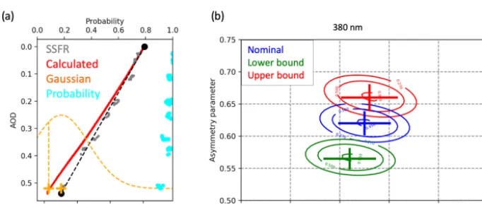
The third step of the retrieval determines the most proba-ble pair of{SSA, g}and calculates the uncertainty. For each
{SSA, g}pair calculation, every SSFR data point in the pro-file is assigned a probability according to the difference be-tween the calculation and the measurement. The probability of{SSA, g}given the SSFR observations is determined from the Gaussian distribution that represents the measurement uncertainty. This is illustrated in Fig. 6a. The probability of that pair given the observations is determined by multiplying the individual probabilities within the profile. The{SSA, g}
pair with the highest probability value is reported as the re-trieval result. The{SSA, g}pair probabilities are shown as a 2-D probability density function (PDF) in Fig. 6b, where the error bars show the 1σ uncertainty for SSA andg sep-arately, determined by the respective marginal (1-D) PDFs. Since only the SSFR uncertainty is considered within the re-trieval, the 4STAR uncertainty is treated separately by per-forming the retrieval three times: (1) for the nominal AOD, (2) for the nominal AOD – range of uncertainty, (3) for the nominal AOD+range of uncertainty. Figure 6b shows an example retrieval at 380 nm for the three retrievals. Finally, the retrieved spectra of 4STAR wavelengths between 355 and 660 nm of SSA andgare reported, with a range of uncer-tainty that encompasses the three separate retrievals.
Currently, the retrieval is performed for each wavelength individually, and no spectral smoothness constraints are ap-plied. This is an important difference compared to other methods such as the AERONET inversion method that re-trieves aerosol size distributions and the real and imagi-nary parts of the index of refraction for various size modes (Dubovik and King, 2000).
Figure 5.The 4STAR homogenized AOD profile for 355 nm is shown as blue circles for(a)20 September 2016 and(b)13 August 2017. The polynomial is shown as a red dashed line, and the derived extinction profile is shown as a teal line. The two black dashed lines indicate the BOL and TOL; any AOD measured above the top of the layer is distributed within a layer up to 15 000 m, well above the spiral altitudes.
Figure 6. (a)This figure shows measurements of downwelling irradiance (gray) along with a calculated profile (red) for one pair of SSA andg. The probability of this pair, given the measurements, is obtained by considering the measurement uncertainty range (represented as a Gaussian, yellow) for the individual data points and assigning a probability (cyan, upper axis) to each data point according to the difference between the calculation and the measurement. The individual probabilities are then multiplied throughout the profile and constitute the probability of the{SSA, g}pair given the observations.(b)shows these probabilities as a function of SSA andg, calculated for the nominal 4STAR AOD (blue) and for the upper (red) and lower (blue) bounds of the reported uncertainty range. The ellipses represent confidence levels of 27 %, 50 %, and 95 %.
(Pilewskie et al., 2003; Bergstrom et al., 2010). The AAE and AAOD are determined as follows:
AAOD=(1−SSA)×AOD, (8a)
AAOD=AAOD500× λ
λ500 −AAE
. (8b)
We compare the AAE and SSA results from our retrieval to in situ measurements from a three-wavelength nephelome-ter (TSI 3563) and a three-wavelength particle soot absorp-tion photometer (PSAP) (Radiance Research). The PSAP provides AAE, while the combination of scattering from the nephelometer and absorption from the PSAP provides
SSA. Average values of SSA are weighted by the extinction, specifically to obtain a column value of SSA from the spiral profiles.
3.3 DARE and critical albedo
We calculate the DARE at the TOL and BOL as the differ-ence between the net irradiance with and without the aerosol layer:
DAREλ=Fλ,netaer−Fλ,netno aer. (9)
with the albedo as measured by SSFR and AOD from 4STAR from a BOL leg. HSRL-2 extinction profiles are taken from the TOL leg (2017) or from the collocated ER-2 leg (2016) to capture any variability within the aerosol encountered along the wall.
Combining vertical and horizontal sampling in this way is predicated on the assumption that the aerosol-intensive properties do not change along the BOL leg, whereas albedo and AOD are expected to vary. This is a reasonable assump-tion as long as the legs do not cross an air-mass bound-ary; in situ measurements show that along the BOL leg on 20 September 2016, the SSA at 530 nm ranges from 0.80 to 0.86 (0.83±0.01, average±standard deviation). During this same time, the PSAP instrument shows that the AAE ranges from 1.71 to 2.02 (1.87±0.05). From a radiation wall leg within the aerosol layer (12:35–12:47 UTC), the SSA ranges from 0.84 to 0.87 (0.85±0.004). The AAE ranges from 1.71 to 1.99 for this time (1.84±0.04). On 13 August (both the northern and southern sections), the SSA from the BOL leg ranges from 0.84 to 0.93 (0.87±0.02), while the AAE ranges from 0.97 to 2.1 (1.6±0.3). Within the aerosol layer (14:08– 14:18 UTC), the SSA ranges from 0.88 to 0.90 (0.89±0.003) and the AAE ranges from 1.80 to 2.16 (1.92±0.07) (Do-bracki et al., 2019). In light of the AAE and SSA ranges in the in situ measurements, it does not appear that the legs crossed an air-mass boundary, but the aerosol-intensive prop-erties also cannot be considered constant. However, the mea-sured variability in the in situ SSA is captured by the standard deviation of its retrieved counterpart and is thus propagated into an uncertainty for DARE.
Since the spectral information is available, we choose to calculate DARE spectrally (350–660 nm) as a percentage of the incoming radiation rather than as broadband values com-monly reported. Within the RTM, the SZA is fixed to the mean value of the above cloud leg; for consistency, SSFR measurements are corrected to this SZA following Eq. (3) (17.9◦for 20 September 2016, 22.1◦ for the North case of 13 August 2017, and 23.2◦ for the South case of 13 Au-gust 2017). The albedo ranges for each case are presented in Table 2, and the aerosol-intensive properties used are pre-sented in Fig. 7. Although 0 and 1 albedo values were not actually encountered, we include them in the RTM runs and calculate the DARE to investigate the behavior at the albedo limits. The relationship between DARE and SSFR-measured albedo is nearly linear; therefore, we fit a line to the 1-D cal-culations to find thexintercept, which is the critical albedo. To estimate the total DARE uncertainty, we combine the errors of the individual components:
δDAREtotal= q
δDAREg
2
+(δDAREalbedo)2
+(δDAREAOD)2+(δDARESSA)2, (10)
where each parameter uncertainty is calculated as
δDAREg=
DAREg+δg−DAREg−δg
2 , (11a)
δDAREalbedo=
|DAREalbedo+δalbedo−DAREalbedo−δalbedo|
2 , (11b)
δDAREAOD=
|DAREAOD+δAOD−DAREAOD−δAOD|
2 , (11c)
δDARESSA=
|DARESSA+δSSA−DARESSA−δSSA|
2 . (11d)
The uncertainties ofg and SSA are obtained from their re-trieval, and the AOD uncertainty is the measurement uncer-tainty. Since the albedo is a ratio of upwelling and down-welling irradiance, calibrated using the same apparatus, the relative precision of the measurements to each other drives the uncertainty rather than through error propagation of each calibrated accuracy. The albedo uncertainty is estimated to be approximately 1 %.
This method assumes all four individual uncertainties are uncorrelated and most likely overestimates the DARE uncer-tainty.
4 Results and discussion 4.1 Aerosol properties
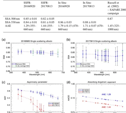
The SSA spectra from 355 to 660 nm retrieved from the radi-ation spirals for each case are shown in Fig. 7a, b, and Table 5 presents a comparison between SSFR-derived SSA and AAE with past results and in situ measurements from ORACLES. The 20 September 2016 case can be considered spectrally flat with a minimum SSA value of 0.83 (±0.02) at 660 nm and a maximum SSA value of 0.86 (±0.01) at 380 nm. The 13 August 2017 case shows a spectrally flat SSA with 0.83 (±0.04) at 355 nm and 0.82 (±0.07) at 660 nm. Compared to the SAFARI 2000 campaign results shown in Russell et al. (2010), the results from the two ORACLES cases are slightly lower, 0.87 at 501 nm compared to 0.85 (±0.01) (20 September 2016) and 0.82 (±0.05) (13 August 2017) at 501 nm, although the values are similar to those presented in Giles et al. (2012) for AERONET sites that experienced smoke aerosol events (Giles et al., 2002; Eck et al., 2003a, b). In situ measurements of the extinction weighted SSA from the spiral profiles and are shown in Fig. 7a, b. At 530 nm, the 20 September 2016 spiral had an average SSA of 0.86 with a standard deviation of 0.03, while the 13 August 2017 spiral had an average SSA of 0.88 with a standard deviation of 0.01. Table 4 presents a comparison at 500 and 530 nm between SSFR-derived SSA and AAE with past results and in situ measurements from ORACLES, and a detailed SSA inter-comparison can be found in Pistone et al. (2019).
Table 5.Comparison of ORACLES SSA and AAE values to Russell et al. (2010) SAFARI results. SSFR results include their estimated uncertainties; the in situ extinction-weighted averages include corresponding standard deviations.
SSFR- SSFR- In Situ- In Situ- Russell et
20160920 20170813 20160920 20170813 al. (2002)
– SAFARI 2000 campaign
SSA-500 nm 0.85±0.01 0.82±0.05 0.87
SSA-530 nm 0.84±0.01 0.81±0.05 0.86±0.03 0.88±0.01
AAE 1.29 (355– 1.44 (355– 1.79±0.15 (470– 1.71±0.07 (470– 1.45 (325–
660 nm) 660 nm) 660 nm) 660 nm) 1000 nm)
Figure 7.Spiral derived SSA values for(a)20 September 2016 and(b)13 August 2017 with associated error bars. The smaller error bars in blue are the spiral uncertainty estimates; the larger error bars (black) are the uncertainties associated with the irradiance pair method. The green symbols show the in situ extinction-weighted average SSA throughout the spiral profile with standard deviations shown as error bars. (c)The retrieved asymmetry parameter with associated error bars for both cases.(d)The AAOD spectra from which the absorbing Ångström exponent is derived for both cases.
be if we had derived the SSA using irradiance pairs rather than from the whole profile (i.e., if the spiral TOL and BOL values had been taken from a radiation wall). The uncertainty derivation for the radiation wall measurements requires the assumption that Hλ=0, though as we have shown, this is
not the case and is described in detail in Appendix A. As can be seen in Fig. 7, the uncertainty from the walls is much larger than from the new spiral method and would be even larger if we included error due toHλ.
Figure 7c shows the asymmetry parameter retrievals along with uncertainty estimates. The values (0.45–0.65) for the 20 September 2016 case are within the range of other esti-mates for the region, although the spectrum falls off more rapidly than assumed by Meyer et al. (2013). The large
campaign for biomass smoke of 1.45 for wavelengths of 325 to 1000 nm. In situ measurements of AAE from the PSAP showed the average AAE values from the two spirals pro-files to be 1.79 for 20 September 2016 and 1.70 13 Au-gust 2017 for the 470–660 nm wavelength range (Dobracki et al., 2019). Differences between radiatively derived and in situ measured values for both AAE and SSA may be due to dif-ferences in aerosol humidification; the irradiances measured by SSFR and the resulting aerosol properties represent the aerosol in ambient conditions (Pistone et al., 2019). The in situ instruments, however, control the relative humidity while the aerosol is measured, potentially causing discrepancies. Biases may also be present in the in situ absorption that prop-agates to bias in SSA, due to known issues with measuring absorption on a filter (Pistone et al., 2019). When the aerosol-intensive properties are derived using our new approach, the aerosol optical properties are radiatively consistent with the measured irradiance and the ambient optical thickness, there-fore allowing us to establish a more direct estimate of DARE. 4.2 DARE and critical albedo
Figure 8a shows the TOL radiative effect as a percent of the incoming radiation at 501 nm as a function of the underlying albedo for 20 September 2016 and the northern and south-ern cases from 13 August 2017. Figure 8b shows example spectra from each case with associated error bars. A positive DARE value indicates that the aerosol warms the layer. For the 20 September 2016 case, the scene albedo, which we con-sider the average of all the albedo values, is 0.5 at 501 nm, with a corresponding TOL DARE of 9.6±0.9 % (percent-age of incoming irradiance). For the 13 August 2017 North case, the scene albedo of 0.03 results in a TOL DARE of
−0.61±2.01 %, while the scene albedo of 0.27 for 13 Au-gust 2017 South results in a TOL DARE of 5.45±1.92 %. As can be seen in Fig. 8, the DARE from the 20 September 2016 case is larger than the 13 August 2016 cases, in large part due to the higher AOD values in the 20 September 2016 case. At the BOL, DARE is always negative since the amount of radiation reaching that altitude decreases when there is an aerosol layer present due to the scattering and absorption that occurs. For this reason, we do not show the BOL DARE re-sults visually. At the scene albedos listed above, the BOL DARE values at 501 nm are−7.27±0.9 %,−8.36±2.01 %, and−4.37±1.92 %, for 20 September 2016, 13 August 2017 North, and 13 August 2017 South, respectively. For the 2017 cases, the clouds were broken on the northern section and homogeneous on the southern section. The TOL radiative ef-fect crosses from negative to positive with increasing albedo, illustrating that the same aerosol has a warming effect in the south and a cooling effect in the north due to the differences in the underlying cloud. This is similar to the conclusions of Keil and Haywood (2003), Chand et al. (2009), and Meyer et al. (2013), who also find that DARE decreases as the un-derlying clouds darken, eventually becoming negative. We
find that the critical albedo is 0.21 at 501 nm for 20 Septem-ber 2016 and 0.26 for 13 August 2017. Chand et al. (2009), along with Meyer et al. (2013) and many other studies, choose to normalize the radiative effect by the aerosol opti-cal depth, a quantity known as the radiative forcing efficiency (RFE), to isolate the cloud effect from the aerosol loading on DARE. For this region, Chand et al. (2009) find that the transition point from positive to negative RFE is at the crit-ical cloud fraction of 0.4. Since we are interested in the ra-diative effects as a function of both the cloud and aerosol properties, we choose not to translate DARE into RFE since it (a) removes the dependence on the aerosol loading and (b) may not linearly scale with mid-visible AOD, with evi-dence suggesting that the increase depends upon the cloud albedo (Cochrane et al., 2019). We can, however, convert critical albedo into critical cloud fraction and critical opti-cal thickness. For a cloud fraction of 100 % and using the two-stream approximation (Coakley and Chylek, 1975), a critical albedo of 0.21 (0.26) corresponds to a critical opti-cal thickness of 1.5 (1.35). Assuming the mean cloud albedo value of 0.5 used by Chand et al. (2009) (determined on the basis of July–October 5◦×5◦ mean and standard deviation of MODIS-retrieved cloud optical depths), a critical albedo value of 0.21 (0.26) and agvalue of 0.56 (0.27) would trans-late into a critical cloud fraction of 0.42 (0.52). This is con-sistent with their finding of the critical cloud fraction to be 0.4. Podgorny and Ramanathan (2001), however, find a much lower critical cloud fraction even with a higher SSA. Chand et al. (2009) attribute this discrepancy to differences in cloud albedo, acknowledging that accurate cloud albedo values are crucial in determining aerosol radiative effects. In reality, one cannot simply fix the cloud albedo to a single value; the true albedo, measured from the BOL leg of the radiation wall, at 501 nm for 20 September 2016 ranges from 0.39 to 0.59, while the 13 August 2016 albedo ranges from 0.06 to 0.39. Using critical albedo instead of critical cloud fraction or op-tical thickness circumvents these problems.
un-Figure 8. (a)The top of layer DARE at 501 nm as a function of the underlying albedo. The critical albedo at 501 nm is 0.2 across all three cases: 20 September 2016 in blue; 13 August 2017 North in purple; 13 August 2017 South in red. The uncertainty estimates are shown for a subset of data points for each case.(b)An example of a DARE spectrum with associated uncertainties for all three cases: 20 September 2016 in blue; 13 August 2017 North in purple; 13 August 2017 South in red. The error bars slightly decrease with increasing wavelength for each case.
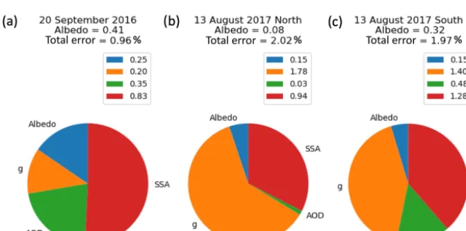
Figure 9.The error contributions ofg(orange), AOD (green), albedo (blue), and SSA (red) for one example each from(a)20 September 2016, (b)13 August 2017 North and(c)13 August 2017 South. Units are the percentage of incident radiation.
certainties. The uncertainty due to the underlying clouds in DARE calculations, while known to be important, is often not emphasized or quantified since the cloud albedo cannot be measured directly from space. Despite the differences be-tween previous studies and our work, the results all high-light the importance for accurate optical properties of both the aerosol and underlying cloud layers, since the radiative effect of an aerosol layer so clearly depends on both.
5 Summary and future work
Aircraft observations, such as those taken during ORACLES, help capture some of the information relevant for determin-ing the aerosol radiative effect in the presence of clouds that satellite measurements are unable to obtain: aerosol SSA,g, and cloud albedo. The aerosol properties, SZA, and albedo
differed between the cases examined in this work, and the critical albedo was 0.21 for 20 September 2016 and 0.26 for 13 August 2017. The critical albedo parameter describes how a certain type of aerosol is affected by the underlying surface despite scene differences. If shown to be applicable across many scenes, this parameter could be very useful for parameterizations of DARE above clouds for biomass burn-ing aerosol.
algorithm allowed us to separate cloud effects from aerosol effects through filtering methods which account for a chang-ing cloud field by eliminatchang-ing regions of high variability and points that are subjected to 3-D effects. We determine this through the H parameter, a proxy for 3-D cloud effects, which is near zero for the filtered spiral measurements but not for the “wall” measurements (stacked legs). The spiral method also considerably decreases the uncertainty on the retrieved SSA compared to the radiation wall method, which is of key importance since the SSA is the largest contributor to the overall DARE uncertainty.
As expected, we found that DARE increases with AOD. However, upon examining other cases (Cochrane et al., 2019), evidence suggests that the increase is not linear with AOD and depends upon the cloud albedo. This puts into question the utility of the concept of radiative forc-ing efficiency that has been widely used in studies such as Pilewskie et al. (2003), Bergstrom et al. (2003), Redemann et al. (2006), Chand et al. (2009), Schmidt et al. (2010a), and LeBlanc et al. (2012). Although these references did not ex-plicitly assume linearity, one must be cautious when using RFE to make the link from satellite-derived optical thickness to DARE. This provides motivation for developing a new approach for establishing such a link, for which the critical albedo could provide that connection as it accounts for both the aerosol and cloud properties.
Future work will also be aimed at verifying whether the DARE–albedo relationship found in this case study is gener-ally valid across scenes with different cloud spatial inhomo-geneities, different sun angles, etc. Work will also be aimed at assessing the remaining suitable ORACLES cases by ap-plying the methodologies presented in this paper to deter-mine regional values of SSA,g, DARE, and heating rate pro-files. The results will be used to parameterize the radiative effects in terms of appropriate quantities such as the AAOD and will be presented in a follow-up paper (Cochrane et al., 2019). It is also important that the SSA be checked for con-sistency with SSA retrieved from other instruments from the ORACLES campaign, such as in Pistone et al. (2019).
Appendix A: Uncertainty estimates
This Appendix describes the full methodology used to obtain the uncertainties presented in the main body of this work. Some equations are repeated from the main body in an effort to make the derivation comprehensible.
The uncertainty analysis provides a way for us to evaluate our absorptance derivation methods and SSA retrieval and to assess whether our DARE calculations are more successful than existing methods. Though we do not use radiation wall irradiance pairs to determine aerosol-intensive properties due to the inability to separateV fromH, we perform the uncer-tainty analysis for illustration only where we must inaccu-rately assumeH=0. We derive the uncertainty for both the radiation wall and spiral methods of finding absorption and propagate those errors into the error of SSA. We assume mea-surements with independent and random uncertainties and therefore propagate errors by adding in quadrature.
A1 Absorptance
The uncertainty on absorptance is calculated from two sep-arate methods: the irradiance pair method, completed using measurements from the radiation wall, and the spiral method which uses data taken only during the aircraft spiral.
The irradiance pairs method relies on determining the ver-tical flux divergence (Vλ) from two collocated irradiance
measurement pairs above and below the aerosol layer (Fλ,↓top, Fλ,↑top, andFλ,↓bot,Fλ,↑bot) following
Vλ=
Fλ,nettop−Fλ,netbot Fλ,↓top
=
Fλ,↓top−Fλ,↑top−Fλ,↓bot−Fλ,↑bot Fλ,↓top .
(A1)
The absorptance would in theory (Song et al., 2016) be found by subtracting the horizontal photon transport fromVλ:
Aλ=Vλ−Hλ. (A2)
We assume thatHλ=0 for the purposes of deriving a
nomi-nal uncertainty value, though this is an inappropriate assump-tion for the condiassump-tions encountered during ORACLES. We have no way of correcting forHλ, and therefore the
follow-ing calculations represent the nominal case where cloud vari-ability has no effect. With this assumption, the absorptance becomes
Aλ=
Fλ,↓top−Fλ,↑top
−
Fλ,↓bot−Fλ,↑bot
Fλ,↓top
, (A3)
and the uncertainty is calculated as
δAλ=
v u u t
−1 Fλ,↓top
δFλ,↑top !2
+ −1
Fλ,↓top δFλ,↓bot
!2
+ −1
Fλ,↓top δFλ,↑bot
!2
+ −1
Fλ,↓top δFλ,↓top
!2
, (A4)
whereδF is the upper limit of the SSFR radiometric uncer-tainty, 5 %. The uncertainty depends on the magnitude of the downwelling irradiance, which is demonstrated clearly in Fig. A1. At the shorter wavelengths where the incoming spectrum is the largest, the uncertainties are much larger than for the longer wavelengths.
The spiral method is based on many measurements taken throughout the profile of the atmospheric column. We there-fore rely on linearly fitting weighted AOD and irradiance measurements to determine the top of aerosol layer and bot-tom of aerosol layer net irradiances.
The following linear fits determine the irradiance values (upwelling/downwelling) at the top (AOD532= minimum)
and bottom of the aerosol layer (AOD532=maximum):
Fλ↑=a↑λ+bλ↑×AOD532, (A5)
Fλ↓=a↓λ+bλ↓×AOD532, (A6)
whereaλ andbλ are the slope and intercept of the linear fit
lines.
The uncertainties on the weighted fit parametersaλ,bλare
calculated according to
σa=
P
w×(AOD532)2
1 , (A7)
σb=
Pw
1 , (A8)
w= 1
σi2, (A9)
where 1=P w×P
w×(AOD532)2− Pw×AOD5322
and σi represent the measurement error. Therefore, when
substituting these into Eq. (3), the absorptance can be found by
Aλ=
AODmax532 ×(bλ↑−bλ↓) aλ↓ ,
(A10)
and the uncertainty on the absorptance is
δAλ=
v u u t
dAλ
dAODmax532 ×δAOD max 532
!2
+ dAλ daλ↓
×σa,λ↓ !2
+ dAλ
db↑λ
×σb,λ↑ !2
+ dAλ
db↓λ
×σb,λ↓ !2
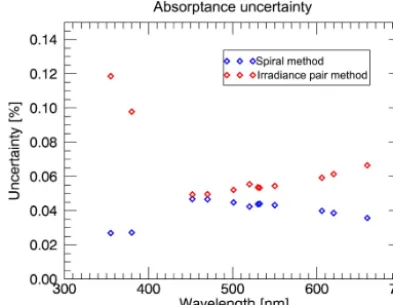
Figure A1. The uncertainty values for the absorptance derivation from the spiral method, shown in blue, and the irradiance pairs method, shown in red, for 20 September 2016. The figure is sim-ilar for 13 August 2017. The uncertainty is significantly reduced with the spiral method, especially at the shortest wavelengths where the incoming irradiance is largest. The uncertainty estimate for the irradiance pairs method depends upon the value of the incoming irradiance, which is largest at the shortest wavelengths.
where σa,b↓,↑ are the uncertainties on the linear fit param-eters. The spiral method compared to the radiation wall method reduces the absorptance uncertainty from 0.05 to 0.02 at 501 nm for 20 September 2016, which is visualized in Fig. A1, and from 0.07 to 0.05 at 501 nm for 13 August 2017. A2 SSA
The SSA retrieval from the spiral measurements produces the uncertainty, while the SSA calculation for the wall illus-tration does not. In order to estimate the uncertainty, we must propagate the absorptance error into the SSA.
To simplify propagation of errors, we determine the rela-tionship between absorptance and AAOD by an exponential fit determined through 1-D radiative transfer calculations: Aλ=c1
1−e−c2×AAODµ λ
, (A12)
whereµ=cos(sza).
The constants c1 and c2 are presented in Appendix
Ta-bles 1a and 2a, and an example of the exponential fit at 380 nm between absorptance and AAOD is shown in Ap-pendix Fig. A2.
Figure A2.Radiative transfer calculations at 380 nm of the relation-ship between absorptance and AAOD. The constant valuesc1and c2for this case at this wavelength are 0.756 and−5.086, respec-tively.
Table A1.Constant valuesc1andc2determined by radiative trans-fer calculations for Eq. (A15) for 20 September 2016.
Wavelength (nm) C1 C2
355 0.797 −2.811
380 0.794 −2.836
452 0.794 −2.794
470 0.797 −2.773
501 0.798 −2.763
520 0.797 −2.77
530 0.797 −2.767
532 0.796 −2.773
550 0.80 −2.75
606 0.805 −2.711
620 0.803 −2.727
660 0.812 −2.666
The AAE and AAOD are determined as follows:
AAOD=(1−SSA)×AOD, (A13a)
AAOD=
AAOD500×
λ λ500
−AAE
. (A13b)
Equation (A12a) can be combined with Eqs. (A13a) and (A13b) and solved for SSA:
SSAλ=1+
µ×ln(1−Aλ
c1)
AODλ×c2
. (A14)