© 2016 IJSRST | Volume 2 | Issue 4 | Print ISSN: 2395-6011 | Online ISSN: 2395-602X Themed Section: Science and Technology
Demodulation of a Single Interferogram based on Bidimensional
Empirical Mode Decomposition and Hilbert Transform
Said Amar
*1, Mustapha Bahich
1, Hanane Dalimi
1, Mohammed Bailich
2, Bentahar Youness
1,
ElMostafa Barj
1, Mohamed Afifi
11Laboratoire d’Ingénierie et Matériaux, Equipe Ingénierie et Energie, Faculté des sciences Ben M'sik, Casablanca, Maroc 2Equipe d’électronique et télécommunications, École Nationale des Sciences Appliquées, Université Mohammed Premier,
Oujda, Maroc
ABSTRACT
The phase calculation is a powerful measurement technique that allows the reconstruction of 3D profiles from interferogram intensity. In this article a new phase extraction algorithm is presented. This algorithm uses the BEMD technique (Bidimensional Empirical Mode Decomposition) for the evaluation of the phase distribution from a single uncarrier interferogram. The proposed method requires the numerical addition of a high spatial frequency carrier and application of the wavelet transform of the Fourier transform. An evaluation was made through a numerical simulation on simulated and real fringes to validate and confirm the performance of the proposed algorithm. The main advantage of this technique is its ability to provide a metrological solution for the fast dynamic analysis.
Keywords:
Interferometry, Fourier Transform, Bidimensional Empirical Mode Decomposition, dynamic
analysis, Carrier Superposition, Phase Retrieval, wavelet transform.
I.
INTRODUCTION
Optical interferometry techniques are widely used as tools for measuring micro-displacement and microstrain in several areas both scientific and industrial. [1]
These non-destructive methods are based on the measurement of small variation of the optical path using interference phenomena. Optical interferometry techniques are many and varied: classical interferometry, speckle interferometry, holography, fringe projection technique, shearography, etc. [2]
The physical quantity to be measured is modulated by a phase which is characterized by a deformed fringe system in an intensity image. The phase extraction algorithms are designed to calculate the phase distribution coding this image [3].
This research is based on the phase extraction from a single uncarrier interferogram using BEMD technique (Bidimensional Empirical Mode Decomposition). We
present here a phase calculation algorithm based on this method for calculating modal intrinsic functions bidimensional (BIMFs) followed by a digital phase shift by Hilbert Transform for each BIMF. Then, a spatial digital carrier has been superimposed followed by an application of the continuous wavelet transform or Fourier transform giving access to the phase distribution across a local analysis of intensity images.
II.
THE EMPIRICAL MODE DECOMPOSITION
The EMD decomposition base is intrinsic to the signal. The extraction of the oscillating components called empirical modes (IMF Intrinsic Mode Functions) is non-linear, but their recombination is linear. As EMD has no analytical formulation, it is defined by an algorithm and a process called sifting [4-6] for decomposing the signal to the Empirical Modes.
To calculate the IMFs of a signal x (t) we follow the following algorithm:
2. Interpolating the maxima sets and the minima sets
(cubic splines, for example), to get the upper envelopes (lower envelopes) :
e
min
t
, emax
t 3. calculate the mean of envelopes:2 ) ( ) ( )
( emin t emax t
t
m
4. subtract the mean envelope of the input signal
)
(
)
(
)
(
t
x
t
m
t
h
5. If h(t) is an IMF, the residue is
r
(
t
)
x
(
t
)
h
(
t
)
and the new signal will be
x
(
t
)
h
(
t
)
,6-If h (t) is not a IMF, the new signal will be
)
(
)
(
t
r
t
x
,For that
h
(
t
)
is a IMF, we must have a extrema between several zero.
extrema
zero
1
and the mean of the upper and lower envelopes is zeroThe signal x (t) can be written as:
nIMF
it
r
t
t
x
1)
(
)
(
)
(
(1)
The scope of the EMD technique to two-dimensional signals (BEMD) follows the same steps for the extraction of the BIMFs and the residue.
III.
HILBERT TRANSFORM
In mathematical and signal theory, the Hilbert transform, denoted H, of a real variable function f (t) is obtained by
convolution of f (t) with
t t h
1 )( [7].
t
d
x
d
t
h
x
t
t
x
t
x
H
(
)
1
(
)
(
)
1
(
)
)
(
(2) Moreover, the Hilbert transform may be interpreted as the output of a invariant linear system as input x(t), which is a impulse response system
t
1
. This is a
mathematical tool widely used in signal theory to describe the complex envelope of the real magnitude modulated by a signal.
Its Fourier transform is expressed as follows:
H
x
(
t
)
H
(
f
)
X
(
f
)
TF
(3)With
(
)
sgn(
)
)
(
f
TF
h
t
j
f
H
(4)Where sgn (f) is the "sign" function such as:
0
,
1
0
,
0
0
,
1
)
sgn(
f
si
f
si
f
si
f
(5)Hilbert transform has the effect of turning of 90° the negative frequency component of x (t) and -90° the positive frequency component. The Hilbert transform does not change the amplitude F (k), it only changes the phase.
Hence the Hilbert transform is equivalent to a filter altering the phases of the frequency components by 90° positively or negatively according to the sign of frequency.
However, the direct application of this transform to interferogram to carry out the phase shift sometimes introduces a sign ambiguity problem can be corrected by a guided method of fringe orientation interferogram [8].
Applying the Hilbert transform to equation (1):
n i i n i it
r
H
t
IMF
H
t
r
t
IMF
H
t
x
H
1 1)
(
(
)
(
)
(
)
(
)
(
(6)Therefore, the Hilbert of a signal x (t) is the sum the Hilbert of all IMF components and the residual r (t). Otherwise, with EMD decomposition (BEMD), we can
shift a signal (image) with
2
.
IV.
THE FOURIER TRANSFORM
The intensity at a point of the interferogram at coordinates (x, y) is expressed as follows:
,
1 ( , )cos
( , )
) ,
(x y I0 x y V x y my x y
I
(7)With, I0, V and are respectively the average intensity,
modulation rate of the high frequency spatial carrier respecting the following condition:
max
y
m
(8)The above expression can be written differently in the following form: imy imy e y x c e y x c y x I y x
I( , ) ( , ) ( , ) *( , )
0 (9)
Where
( , ) 0 2 , ) , ( ) ,(x y I x y V x y ei xy
c (10)
The one-dimensional Fourier transform is performed on Equation (7) along the line x. The spectrum of the thus obtained interferogram is expressed as:
)
,
(
ˆ
)
,
(
ˆ
)
,
(
ˆ
)
,
(
ˆ
*0
x
k
C
x
k
m
C
x
k
m
I
k
x
I
(11)Where
I
ˆ
,I
ˆ
0 ,C
ˆ
andC
ˆ
* are respectively the Fourier Transform of I , I0 , c and c*
After filtered two components
I
ˆ
0 andC
ˆ
*, and shifted the componentC
ˆ
to the origin. The inverse Fourier transform is applied toC
ˆ
for obtain c (x, y).The real and imaginary parts of c (x, y) are given by
(
,
)
(
,
)
cos(
(
,
))
Re
c
x
y
b
x
y
x
y
(12)
(
,
)
(
,
)
sin(
(
,
))
Im
c
x
y
b
x
y
x
y
(13)The desired phase distribution will be evaluated using the arctangent of the quotient Equation (13) on Equation (12):
) , ( Re ) , ( Im ) , ( y x c y x c arctg y x
(14)V.
THE CONTINUOUS WAVELET TRANSFORM
(CWT)
Unlike the overall processing the Fourier analysis, the wavelet transform allows a local study of the optical information modulating the interference signal I(x, y).
By applying the wavelet transform to signal I(x,y), we will have:
I
x
y
y
dy
b
a
x
W
(
,
,
)
(
,
)
a*,b(
)
(15)Where
a,b are the wavelets: very special elementaryfunctions constructed from the wavelet mother
(
y
)
by translation and dilation [4-6] such as:
a
b
y
a
y
b a
,(
)
1
(16)
Where a0 : The dilation parameter (scale) and b: the translation parameter. Therefore
I x y V x y my
a b a x
W( , , ) 1 0( , )1 ( , )cos( (17)
Exploiting the localization of the wavelet and assuming a slow variation of I0 and V, the Parseval identity leads
to
( , ) * ) , ( * 0ˆ
ˆ
2
)
,
(
)
,
(
)
,
,
(
b x i b x ie
y
m
a
e
y
m
a
a
b
x
V
b
x
I
b
a
x
W
(18)) , ( * 0
ˆ
2
)
,
(
)
,
(
)
,
,
(
b x i
e
y
m
a
a
b
x
V
b
x
I
b
a
x
W
(19)
The modulus and the phase arrays can be calculated by the following equations:
)
,
(
)
,
(
a
b
W
a
b
abs
(20)
)) , ( Re(
)) , ( Im( arctan )
, (
b a W
b a W b
a
(21)To compute the phase of the row, the maximum value of each column of the modulus array is determined and then its corresponding phase value is found from the phase array [9]. By repeating this process to all rows of the fringe pattern, a wrapped phase map is resulted and needs after to be unwrapped [10].
VI.
INTERFEROGRAM ANALYSIS
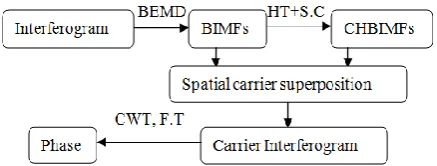
Our method of analysis of an interferogram can be outlined by the following chart (Figure 1)
Figure 1: The flow chart of interferogram analysis method
After applying the BEMD on our interferogram, we get the BIMFs, on which we apply the Hilbert Transform to
digitally shift with
2
. These shifted BIMFs will be later
corrected to remove their sign ambiguity and the new images are called CHBIMFs.
By adding all BIMFs and CHBIMFs, we find the two BIMF and CHBIMF images respectively.
Using a suitable modulation rate m, we combine digitally SIMF(x,y) and CHBIMF(x,y) with the matrix
cos(my) and sin(my) to derive the carrier interferogram IP as following :
)
,
(
)
sin(
)
,
(
)
cos(
)
,
(
y
x
SCHIMF
my
y
x
SIMF
my
y
x
IP
(22)
By using the Fourier Transform or wavelet Transform, we can obtain simply the phase distribution.
VII.
SIMULATIONS AND RESULTS
In this work, we apply our algorithm on an interferogram with size 256 × 256 pixels whose distribution is given by:
(
,
)
cos
1
)
,
(
x
y
x
y
I
(23)
and illustrated in figure 2
Figure 2: The simulated interferogram
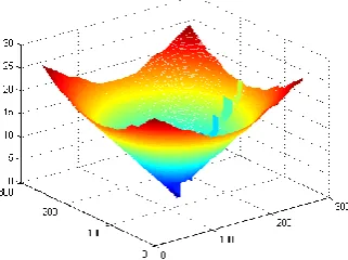
with ϕ(x,y) the phase variation that have expression:
2
2128
128
15
.
0
)
,
(
x
y
x
y
(24)
shown in Figure 3
Figure 3: The theoretical phase distribution With x and y are the pixel coordinates in the image
Figure 4: BEMD decomposition of interferogram (BIMFs)
After that, the Hilbert Transform is applied to each BIMF followed by a sign correction. Figure 5 shows the sum of all corrected BIMFs. It’s a π/2 phase shifted interferogram.
50 100 150 200 250
50
100
150
200
250
Figure 5:
2
phase shifted interferogram.
After combining the two phase shifted fringe patterns numerically with sin (my) and cos (my), we have obtained the modulated fringe pattern shown in Figure 6 with modulation rate value 0.8 radian/pixel.
50 100 150 200 250
50
100
150
200
250
Figure 6: The carrier interferogram
The wavelet method was applied to the new carrier fringe pattern to retrieve the phase map of Figure 7.
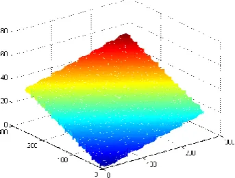
Figure 8 illustrates the retrieved continuous phase map after the unwrapping process.
50 100 150 200 250
50
100
150
200
250
Figure 7: The wrapped phase map
Figure 8: The retrieved phase map
VIII.
APPLICATION ON REAL FRINGES
To illustrate the use of our method for real applications, we tested its performance on a rough ground finish, aluminium surface from a hard disk drive assembly of the company 4D Technology.
Figure 9 shows the real fringes of Hard Drive at aluminum.
Figure 9: Real fringes of the hard drive enclosure By applying the same steps as before, we find the wrapped phase distribution by using the Fourier Transform (FT) (Figure 10):
50 100 150 200 250
50
100
150
200
250
Figure 10: The wrapped phase by F.T
Figure 11 shows the distribution of the continuous phase obtained after unwrapping process.
Figure 11: The unwrapped phase distribution by F.T And if using the continuous wavelet transform (CWT), we find the wrapped phase distribution shown in figure 12.
50 100 150 200 250
50
100
150
200
250
Figure 12: The wrapped phase by CWT.
The figure 13 shows the distribution of continuous phase after unwrapping method.
Figure 13: The unwrapped phase distribution by CWT with both methods we obtained the same phase
distribution
IX.
CONCLUSION
In this paper, we have presented a new algorithm of phase retrieval from a single uncarrier interferogram with closed fringes. This was achieved by numerical superposition of the spatial carrier by Empirical Mode Decomposition and Hilbert Transform, followed by fringes demodulation using Continuous Wavelet Transform or Fourier Transform.
The numerical simulation validated the reliability of the method on simulated and real fringes by estimating the phase distribution with good accuracy even with the closed fringes.
X.
REFERENCES
[1] D.C. Williams, "Optical methods in engineering metrology". Chapman and Hall, First edition. (1993).
méthode des champs virtuels, PhD thesis, École Nationale Supérieure d’Arts et Métiers, 2007. [3] M. Afifi, these d’état, Université Hassan II
Mohammedia, (2002).
[4] N. E. Huang, Z. Shen and S. R. Long, ''The empirical mode decomposition and the Hilbert spectrum for nonlinear and non stationary time series analysis'' in: Proceedings of the Royal Society of London Series, 1998, 454, pp. 903- 995.
[5] G. Rilling, P. Flandrin, “On empirical mode decomposition and its algorithms”, in: IEEE– EURASIP Workshop Nonlinear Signal Image Process, Grado, Italy, 2003.
[6] Cexus Jean-Christophe, " Analyse des signaux non stationnaires par Transformation de Huang,Opérateur de Teager-Kaiser, et Transformation de Huang-Teager (THT) " these de Doctorat, 2005.
[7] EB Saff, AD Snider, “Complex analysis for mathematics, science and engineering”, Prentice- Hall Inc, New York, (1976).
[8] M Bahich, M Afifi, EM Barj, “Optical phase extraction algorithm based on the continuous wavelet and the Hilbert transforms”, Journal Of Computing, vol.2, 5, (2010)
[9] Q. Kemao, et al., Wavelets in optical metrology, in: K. Singh, V.K. Rastogi (Eds.), Perspectives in Engineering Optics, 2003, pp. 117–133.