Image Restoration Based on Deconvolution by Richardson Lucy Algorithm

ISSN: 2231-5381

http://www.ijettjournal.org

Image Restoration Based On Deconvolution by

Richardson Lucy Algorithm

Madri Thakur#1, Shilpa Datar*2

#1

PG student, Dept. of Electronics and CommunicationEngg. SATI, Vidisha, M.P., India

*2

Asst. Prof., Dept. of Electronics and Instrumentation Engg SATI, Vidisha, M.P., India

Abstract— This article presents the performance analysis of different basic techniques used for the image restoration. Restoration is a process by which an image suffering from degradation can be recovered to its original form. Removing blur and noise from image is very difficult problem to solve. We have implemented the three different techniques of image restoration and tested our implementation for the blurred image in the standard environment. We have obtained the blurred image with the standard blurring functions and the noise. The degraded images have been restored by the use of Wiener deconvolution, Inverse deconvolution and Richardson–Lucy algorithm. Further we have compared the different results on the basis of PSNR and MSE values of the restored image. Finally the conclusion is formulated.

Keywords— Inverse filter, Wiener filter, Lucy- Richardson, MSE (mean square error), PSNR (peak signal to noise ratio).

1.INTRODUCTION

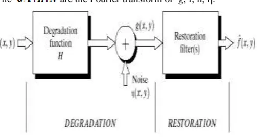
The task of deblurring, a form of image restoration, is to obtain the original, sharp version of a blurred image.[1-3] There exist many applications for image restoration, including astronomical imaging, medical imaging, law enforcement, and digital media restoration. The problem has attracted strong research interest and will continue to do so, not only because it has many applications but also because it has a simple mathematical formulation yet it is a classical inverse problem for which good solutions are not easily obtained. The simple equation for expressing image blurring/degradation is as follows;

g = f * h + η (1)

Where f is the original image and g is the version that has been degraded through blurring (convolution ∗) by kernel h and the addition of random noise η. This degradation model represents a linear relationship between f and g; hence, the problem of recovering f from g is called linear

image restoration. Often the blur kernel is assumed to be space-invariant [4-5]. If we lack prior knowledge of the blur kernel or point spread function h, we have the more difficult blind (linear) image restoration problem in which h also needs to be estimated. Also we have

G (u) = F(u)H(u) +N(u) (2)

The are the Fourier transform of g, f, h, η.

Fig. 1 Image Blurring model

Image deconvolution methods are used to estimate the latent image from the degraded image. They can be divided into two categories, non-blind and blind deconvolution [6-7]. In non-blind deconvolution, the PSF is known and f can be restored through an error.

Minimization process. The Weiner deconvolution and the Inverse deconvolution are the two commonly used methods, within this category.

Richardson–Lucy deconvolution is

ISSN: 2231-5381

http://www.ijettjournal.org

3. INVERSE DECONVOLUTION METHOD FOR IMAGE DEBLURRING

Direct inverse Filtering is the simplest approach to restoration [9]. In this method, an estimate of the Fourier transform of the image (u, v) is computed by dividing the Fourier transform of the degraded image by the Fourier transform of the degradation function

(u, v) = G (u, v) / H (u, v) (3)

This method works well when there is no additive noise in the degraded image. That is, when the degraded image is given by

g(x, y) = f(x, y)*h(x, y) (4)

But if noise gets added to the degraded image then the result of direct inverse Filtering is very poor. Equation 1.gives the expression for g(u, v). Substituting for G(u, v) in the above equation, we get

(u, v) = F ((u, v) + N(u, v)H(u, v) (5)

The above equation shows that direct inverse Filtering fails when additive noise is present in the degraded image. Because noise is random and so we cannot find the noise spectrum .

Fig. 2 Inverse Deconvolution

4. WEINER DECONVOLUTION METHOD FOR IMAGE DEBLURRING

Weiner deconvolution is named after Norbert Weiner, who first proposed the method in 1942 w Weiner filtering is one of the earliest and best known approaches to linear image restoration [9].

Weiner Filtering is more robust in the presence of additive noise. Weiner filtering incorporates both degradation function and statistical characteristics of noise into the restoration process. The objective of this technique is to find an estimate of the original image f such that the mean square error between them is minimized. This error measure is given by

(6)

Where E{.} is the expected value of the argument. The method is founded on considering image and noise as random processes and objective is to find an estimate of the uncorrupted image such that the mean square error between them is minimized. If the noise is zero, then the noise power spectrum vanishes and the wiener filter reduces to the inverse filter.

5. RICHARDSON–LUCY DECONVOLUTION ALGORITHM

The non blind convolution is the category of de-convolution method in which the PSF is known. The Richardson–Lucy deconvolution algorithm has become popular in the fields of astronomy and medical imaging. Initially it was derived from Bayes theorem in the early 1970’s by Richardson and Lucy. In the early 1980’s it was redeliver by Shepp and Vardi as an algorithm to solve positron emission tomography imaging problems, in which Poisoning statistics are dominant. Their method used a maximum-likelihood solution, which was found by use of the expectation maximization algorithm of Dempster et al

} ) f -E{(f

e 2

ISSN: 2231-5381

http://www.ijettjournal.org

Richardson–Lucy algorithm is its implementation of maximum likelihood and its apparent ability to produce reconstructed images of good quality in the presence of high noise levels. We therefore assumed that a non blind form of this algorithm would have the same characteristics [2-6].

Non linear iterative technique is better than the linear technique. Non linear behaviors is not always predictable and required computational resource’s-R algorithm which is arise from the maximum like hood formulation

(7)

6. RESULTS AND ANALYSIS

Where is the convolution operation. F= is the estimate of the un degraded image. We have used the R-L algorithm iteratively staring from the blurred image. The image restored after each iteration moves closer to the original image thus reducing MSE with number of iterations. The program execution is terminated when MSE obtained becomes constant in consecutive iterations

7. PERFORMANCE PARAMETERS

Image restoration research aims to restored image

to from a blurred and noisy image A widely used measure of reconstructed image

fidelity for an N * M size image is the mean square error (MSE) and is given by –

We have evaluated the results for different images .The results are shown for the two images for the different variance and image sizes.

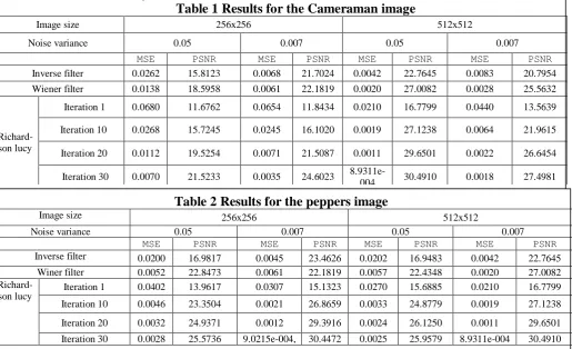
Table 1 Results for the Cameraman image

Image size 256x256 512x512

Noise variance 0.05 0.007 0.05 0.007

MSE PSNR MSE PSNR MSE PSNR MSE PSNR

Inverse filter 0.0262 15.8123 0.0068 21.7024 0.0042 22.7645 0.0083 20.7954

Wiener filter 0.0138 18.5958 0.0061 22.1819 0.0020 27.0082 0.0028 25.5632

Richard-son lucy

Iteration 1 0.0680 11.6762 0.0654 11.8434 0.0210 16.7799 0.0440 13.5639

Iteration 10 0.0268 15.7245 0.0245 16.1020 0.0019 27.1238 0.0064 21.9615

Iteration 20 0.0112 19.5254 0.0071 21.5087 0.0011 29.6501 0.0022 26.6454

Iteration 30 0.0070 21.5233 0.0035 24.6023

8.9311e-004 30.4910 0.0018 27.4981

Table 2 Results for the peppers image

Image size _{256x256 512x512}

Noise variance 0.05 0.007 0.05 0.007

MSE PSNR MSE PSNR MSE PSNR MSE PSNR

Inverse filter _{0.0200 16.9817 0.0045 23.4626 0.0202 16.9483 0.0042 22.7645}

Winer filter 0.0052 22.8473 0.0061 22.1819 0.0057 22.4348 0.0020 27.0082

Richard-son lucy

Iteration 1 0.0402 13.9617 0.0307 15.1323 0.0270 15.6885 0.0210 16.7799

Iteration 10 0.0046 23.3504 0.0021 26.8659 0.0033 24.8779 0.0019 27.1238

Iteration 20 0.0032 24.9371 0.0012 29.3916 0.0024 26.1250 0.0011 29.6501

Iteration 30 0.0028 25.5736 9.0215e-004, 30.4472 0.0025 25.9579 8.9311e-004 30.4910

y)] (x, f * y) y)/h(x, g(x,

* ) y)[h(-x,-y (x,

f y) (x, f

_k

^ k

^ 1

k ^

ISSN: 2231-5381

http://www.ijettjournal.org

original image image affected by blurring

50 100 150 200 250 50

100

150

200

250

(a)image restore by weiner filtering (b)

50 100 150 200 250 50

100

150

200

250

image restore by Inverse filtering

50 100 150 200 250 50

100

150

200

250

(b) (d)

restored image after the itrretion 30

50 100 150 200 250 50

100

150

200

250

(e)

Fig.3 Results of pepper.png (a) original image (b) blurred image (c) Restored by Inverse filter (d) Restored by Wiener filter (e)Restored by R-L at iteration 30.

From Fig.(3) (c) & (d), and Fig.4 (c) & (d), the above results we found that the inverse filter works better than the Weiner filter, under noise conditions. When the variance of noise increases the performance of inverse filtering not provides the sufficient PSNR. The Weiner filtering gives the good PSNR regardless of the noise variance

Form Fig.3 (e) and 4 (e), the results obtained by the Richardson Lucy method, we have found that the PSNR increases with the number of iterations and also the quality of the image enhances.(See Table 1 and 2).

original image

image affected by blurring

50 100 150 200 250 50

100

150

200

250

(a) (b)

image restore by Inverse filtering

50 100 150 200 250 50

100

150

200

250

image restore by weiner filtering

50 100 150 200 250 50

100

150

200

250

(b) (d)

restored image after the itrretion 30

50 100 150 200 250

50

100

150

200

250

(e)

Fig.4 Results of cameraman.tif (a) original image (b) blurred image (c) Restored by Inverse filter (d) Restored by Wiener filter (e)Restored by R-L at iteration 30.

8. CONCLUSION

We have seen the requirement and significance of image de-blurring. We have seen the mathematical formulation for the blurred image. we already have the knowledge of point spread function .

Weiner filtering provides the better results than the inverse filtering almost in every condition except when the noise having very less variance.

The Richardson Lucy provides good estimate for the blurring function and gives better PSNR within the limited iterations. Yet if we use this method with the known point spreading function then it is a time taking method, still it can provides the PSNR even better than Weiner deconvolution.

ISSN: 2231-5381

http://www.ijettjournal.org

deconvolution.

REFERENCES

[1] J. G. Walker, D. A. Fish, A. M. Brinicombe, and E. R. Pike, “Blind deconvolution by means of the Richardson–Lucy algorithm”J. Opt. Soc. Am. A, Vol. 12, No. 1, January 1995.

[2] Arijit Dutta, Aurindam Dhar, Kaustav Nandy, Project report on “Image Deconvolution By Richardson Lucy Algorithm”, Indian Statistical

Institute, November, 2010.

[3] G. R. Ayers and J. C. Dainty, “Iterative blind deconvolution method and its applications,” Opt. Lett. Vol.13, 547–549 , 1988 .

[4] J. R. einup, “Phase retrieval algorithms: a comparison,” Appl. Opt.

Vol.21, 2758–2769, 1982.

[5] B. L. K. Davey, R. G. Lane, and R. H. T. Bates, “Blind deconvolution of noisy complex-valued image,” Opt. Commun. Vol.69, 353–356, 1989.

[6] W. H. Richardson, “Bayesian-based iterative method of image restoration,” J. Opt. Soc. Am. Vol.62, 55–59 1972.

[7] L. B. Lucy, “An iterative technique for the rectification of observed distributions,” Astron. J. Vol. 79, 745–754, 1974.

[8] Ramesh Neelamani, Thesis report on “Inverse problems in image processing” Electrical and Computer Engineering Rice University, Houston, Texas.

[9] Reginald L. Lagendijk and Jan Biemond, “Basic methods for image restoration and Identification”, Lagendijk- Biemond, February, 1999.