INTERNATIONAL RESEARCH JOURNAL OF PHARMACY
www.irjponline.com
ISSN 2230
–
8407
Research Article
BACKGROUND NORMALIZATION AND TEXTURE PATTERN-BASED VIDEO SEGMENTATION FOR VISUAL TRACKING
V.Rajagopal 1*, B.Sankaragomathi 2
1Department of Electronics and Communication Engineering, MET Engineering College, Kanyakumari, Tamil Nadu, India
2Department of Electronics and Instrumentation Engineering, National Engineering College, Tuticorin, Tamil Nadu, India
*Corresponding Author Email: [email protected]
Article Received on: 19/10/17 Approved for publication: 19/11/17
DOI: 10.7897/2230-8407.0811239
ABSTRACT
Visual tracking is the task of estimating the path of a target object in each frame of the video. Various tracking approaches are developed for tracking the position of the target. However, the tracker may fail to find the correct position, if the appearance of the target is similar to the background. This paper proposes a background normalization technique based on the textural pattern analysis to verify the matching of the features for the target region analysis. In this work, a novel model of background clustering is presented by using Multi-Weighted Chain Prediction (MWCP) algorithm for the uneven background. A Neighborhood Differential Binary Pattern (NDBP) is proposed to extract the texture for suppressing the shadow pixels in the image frame. From this equalized frame of the given video, the frame is split into several grids. From the grid format frame, the histogram features of the targeted frame are extracted, and each grid in that frame is classified. The Multi-Grid Weighted Classifier (MGWC) algorithm is used to find the matching of the grids to separate the background and foreground. This type of visual tracking system is robust over the sudden illumination changes and dynamic background. The experimental result proves that the proposed approach yields better precision, recall and F-score performance than the existing tracking approaches.
Keywords: Background Normalization, Histogram Features, Texture Pattern, Video Segmentation, Visual Tracking System
INTRODUCTION
In the real-time application, most of the research works focus in the visual tracking system (1), (2), (3), (4), (5), (6). It is mainly used in the application such as robotics, visual surveillance (7), Human-to-Machine Interface (HMI) (8), video editing (9), motion control (10), (5), (11), (12), and activity recognition (6) to extract the target status. There are number of visual tracking systems to identify the targeted region from the frame of a given video. But, the tracking performance can be affected by the sudden illumination changes (13), shadowing effect and uneven background. In the moving object detection system, it suffers from the change in the dynamic background and presence of shadow effect in the video frames. Due to this, there occurs misclassification in the tracking of targeted region. It results in the false detection of moving objects. To rectify this problem, the researchers developed many techniques such as K-Means clustering, Fuzzy C-Means, etc. to detect and eliminate the shadow from frames. These techniques are used to segment both the foreground and background from each frame. Then, they remove or suppress shadow region and track the target. In these methods, the segmentation is based on the static background of the surveillance area.
Motivation
The features play a significant role in the object recognition. But, the features are defined and combined manually in many online visual tracking systems (14), (15), (16), (17), (18), (19), (20). However, these methods yield satisfactory results on the individual datasets, the feature representations limit the tracking
performance. The normalized cross correlation will be discriminative during the favorable lighting conditions. But, it is ineffective if the object moves under the shadow. This requires better learning mechanisms for capturing the effective change in the appearance with respect to time. The state-of-the-art approaches focus on the extraction of local binary patterns (21), Haar-like features (17), (22), (23), histograms (4), (24), HOG descriptors (19), and covariance descriptors (25). However, these approaches require the learning techniques to improve the representative capabilities. The texture is a property that defines a way for changing the color in the neighborhood of the pixels (26). The texture for the target object and background having the same color is different. The Local Binary Patterns (LBP) is a simple description operator for the local texture (26), (27). Due to the low computational complexity and better ability for coding the details, the LBP is widely used in object tracking (28), (29).
Proposed work
classify each grid in that frame. The MGWC algorithm is used to find the matching of the grids. The matching grid is considered as the tracked region, and a binary label is provided to the matched grid to separate the background and foreground. This type of visual tracking system is robust over the sudden illumination changes and dynamic background by using the texture pattern analysis.
Organization of the paper
The remaining sections in the paper are structured as follows: Section II describes a brief overview of the current research works related to the video segmentation and target tracking approaches. Section III explains the proposed video segmentation approach including the median filtering, MWCP, NDBP and MGWC algorithms. Section IV presents the performance analysis including the dataset description, comparative analysis with the existing tracking approaches and tracking analysis. Section V includes the conclusion and future scope of the proposed video segmentation approach.
RELATED WORK
Babaee et al. (30) proposed an approach for tracking the superpixels associated within each box in the multi-view video sequences. A flow graph was constructed, and both the visual and geometric cues were combined in the global optimization framework. Hence, the segmentation, reconstruction, and tracking of the target objects in the video were performed simultaneously. Wang et al. (31) introduced an accurate method for recovering the individual trajectory of each active colloid. A level set method was applied for the segmentation of the individual colloid. The trajectories of the colloids were recovered concurrently as vertices on the weighted graph. Liwicki et al. (32) developed a Kernel Slow Feature Analysis framework for the temporal-based video segmentation and target tracking. The proposed approach improved the tracking setup while combining with the online learning tracking system. Xiaojun et al. (33) presented an enhanced active contour model algorithm for tracking the moving objects. From the detection result of the frame difference, the coarse contour of the moving target was found out, and convergence of the contour was performed to achieve tracking of the moving object. Drayer and Brox (34) introduced an approach for the object segmentation in videos that combines the frame-level object detection with the object tracking and motion segmentation concepts. An accurate and temporally consistent segmentation of each object was provided. The performance was reduced due to the missing annotation of static objects and labeling of different objects as a moving object. Khoreva et al. (35) suggested an approach for video segmentation by focusing on the superpixel. Keuper and Brox (36) addressed the problems in the segmentation of temporally consistent boundary and hierarchical video segmentation. The temporally consistent boundaries were the key components for the assignment of temporally consistent region. The proposed method was independent of the optical flow computation or previously learned motion models. The segmentation quality was lower than the quality obtained with the multiscale approach. Spina and Falcão (37) applied spatiotemporal superpixel-graph for interactive video segmentation. The segmentation of the second frame was refined by limiting the delineation on the pixel-graph within the expected boundary region of the object. However, the weight computation process was slow and expensive. Jiang et al. (38) presented a novel framework for the spatiotemporal segmentation of the video sequence. An iterative optimization scheme was introduced through the independent initialization of the segmentation maps for each frame. The proposed framework produced unsatisfactory segmentation
results due to the difficulty in handling the problems of a large number of occlusions or out-of-view. Cao et al. (37) proposed an object-level method for extracting the foreground object in the video. The proposed method guaranteed the continuity of segmentation result and exhibited better performance even during the fast motion and presence of occlusion.
Li et al. (39) introduced an efficient approach for video segmentation while reducing the effect of data noises and corruptions. The proposed approach suffered from the low segmentation quality due to the sensitivity to the noise and corruptions. Chen et al. (40) proposed a novel approach for the segmentation of a moving object in the video by using the point trajectories. A graph-based segmentation was introduced by adopting the local and global motion information encoded by the trajectories of the tracked dense point. However, this approach does not work well for the object without distinct motions from the background in various scenes. Delibasis et al. (41) presented a novel algorithm for the accurate segmentation of foreground in the video sequences. The proposed method was capable of handling the sudden changes in the light obtained from the natural and artificial light sources. Gangapure et al. (42) proposed a novel framework for the segmentation of causal video using the superseeds and graph matching. Finally, the watershed algorithm was applied to achieve final video segmentation. Wang et al. (43) presented a semi-supervised approach for the segmentation of semantic video object with respect to the variations in the shape, appearance, and presence of an obstruction in the video. This approach was highly sensitive to the motion accuracy. Abdelwahab et al. (44) proposed a method for the segmentation of video object by using the motion of superpixel centroids. After the segmentation of each object, the foreground objects, and the background were distinguished by using the clustering results. Husain et al. (45) developed an approach for the segmentation of Three-Dimensional (3D) point clouds into the geometric surfaces by using adaptive surface models. An adaptive mechanism was included for the construction and removal of the segments. But, the segment overlapping between the consecutive frames is to be reduced. Molina-Giraldo et al. (46) proposed a video segmentation framework for detecting the moving objects in a scene. A tuned K-means technique was used for grouping the pixels as static or moving objects. The proposed framework was tested to classify the people and abandoned objects. However, it does not support the actualization of the background model. Li et al. (47) presented a single Convolutional Neural Network (CNN) based tracking algorithm for the effective online learning of the feature representations of the target object. Razavi et al. (48) introduced a texture-based target representation and suggested an improved mean shift tracking algorithm by using the modified Interlaced Derivative Pattern (IDP) that considers the three-dimensional dependencies between the pixels. To overcome the existing issues, video segmentation based on the background normalization and target pattern analysis is proposed.
PROPOSED METHOD
Target matching is the analysis of the movement of a particular target object. The previous target tracking algorithms use template matching. It finds the correlation between the present frame and target. Highest matching of the region in the matrix is determined as a matching region. But, it does not retrieve the proper results. If a specific region is segmented, the segmented region is compared with the target by using the structural information and intensity variations of the target.
The matching of the feature in the grid is determined as a region matching. Previously, a maximum number of features are obtained from the Gabor, correlated values, and sparse representations. In a football match video, the face of the players can be tracked. But, there exist background variations in each frame. In the existing works, the target is fixed at the first frame,
and it is not updated at the next frames. The structure of the target varies with the progress of the frames. As the position of the target changes in each frame, the existing works cannot retrieve the target properly due to the improper matching of the structures. Hence, there is a need to update the position of the target for achieving better tracking performance.
Figure.1 Overall flow diagram of the proposed background normalization and texture pattern based video segmentation approach
In our proposed work, the patterns are used for the target matching analysis. The matching of the extracted patterns with the target patterns is verified by using a simple classifier. The classifier determines the likelihood of the extracted patterns and target patterns. The patterns are extracted grid-by-grid. The size of the grid corresponds to the size of the target to obtain the relevant tracking results. The weight value of each grid is estimated. But, the weight value changes in each frame. So, the weight values are to be updated properly along with the target. If a target is tracked, the tracking region is updated as a target.
This paper proposes a video segmentation approach based on the background normalization and textural pattern analysis. Initially, the video frame is preprocessed. The MWCP algorithm is applied for the background clustering. Then, the NDBP patterns are extracted to suppress the shadow pixels in the frame. The video frame is split into several grids and pixel weight of each grid is estimated. The connecting components are extracted. The video data is preprocessed, and training features are applied. The MGWC algorithm is applied for finding the matching of the grids. A binary label is assigned to the matched grid and blob is extracted for tracking the target. Figure.1 shows the overall flow
diagram of the proposed background normalization and texture pattern-based video segmentation approach for visual tracking.
Median filtering
The input image is preprocessed for removing the noise present in the image by using a median filter. The median filtering is a non-linear approach used for removing the noise such as salt and pepper noise from the images while preserving the edges. This filter moves through the entire image in a pixel-by-pixel manner and replaces each pixel value with the median value of the neighboring pixels. In this technique, the window is formed based on the neighboring patterns, then its median value is calculated by sorting all pixels. Also, the size of window is initialized as
3 × 3, and it is projected over the rows and columns of the matrix. Finally, the pixel values are sorted based on the variation in the neighboring pixels. If the sorted value lies within the specified range, the denoised frame is obtained based on the filtering coefficient. If the sorted values of the window matrix for varying direction ‘𝜃’ of the neighborhood values is greater than the median value, the neighborhood pixels are updated. From this filtering algorithm, we retrieve the pre-processed video frame for both message frame and cover frame.
Algorithm 1: Median Filtering Algorithm
Input: Testing Frame – Y Output: Denoised Frame – Y
i, j – Row and Column iteration respectively. Step 1: Initialize window size (3×3)
Step 3: Initialize filtering coefficient 𝐶 = 𝑚𝑒𝑑𝑖𝑎𝑛(𝑇) Step 4: Check neighboring pixel variation
Step 5: S = sort (T);
Step 6: if𝑆(𝑁𝑒𝑖𝑔ℎ𝑏𝑜𝑟ℎ𝑜𝑜𝑑) == {0 & 255}
Step 7: Y(i, j) = C; Step 8: end if
Step 9: if{𝑆𝜃} > 𝐶
Step 10: Y(i, j) = Y(i, j-1); Step 11: end if
The median values are extracted, and the noisy conditions of the neighborhood regions are checked based on the specified range 0 to 255. If the neighborhood regions are noisy, the median value is replaced in the center pixel. If the noisy level is in the different range with respect to the center pixel, the pixel value of the nearest neighborhood is replaced in the center pixel. The same variable ‘Y’ is used for both input and denoised frame for updating the noise removal in the input frame. If a separate variable is used, the noise is removed in the output frame and not removed in the input frame. The previous noise remains as such.
If it is compared with the nearest neighborhood, there is a possibility of a noisy pixel to be a noise-free pixel. Hence, the noise removal is performed in the input frame. The performance of the median filter is compared with the Gaussian filter and average filter. Figure.2 shows the initial frame of the cup, basketball, and David datasets, which are obtained from this (49). Figure.3 illustrates the comparison between the filtered results of cup, basketball and David datasets obtained from the (a) average filter, (b) Gaussian filter and (c) median filter.
Figure.2 Initial frame of cup, basketball and David datasets
(a) (b) (c)
MWCP
The camera tilts with the movement of the target. Hence, there is variation in the background region. The MWCP algorithm is used for removing the uneven background and eliminating the irrelevant data corresponding to the target. An image frame may contain multiple regions that are relevant to the target. The regions having same intensities and patterns with respect to the target are grouped, and the irrelevant regions are removed. It is termed as background clustering. The irrelevant regions are considered as background. Only the relevant data is retrieved as a cluster from the image frame. The remaining data is formed as a separate cluster.
The input frame ‘Y’ is applied as an input to the MWCP algorithm. The background and foreground regions are extracted as separate clusters, and the clustering index is obtained for the
regions. The Linear of Gradient (LOG) distribution is obtained by using the Gaussian Kernel ‘G’. As the Gaussian Kernel has zero mean and equal variance, it is used. The input frame and target image are convoluted with the LOG distribution to obtain the patterns clearly and likelihood for the efficient separation of the background and foreground regions. Otherwise, the background region may be similar to the foreground region. The matching regions in the frame are extracted as template regions. The template regions having maximum likelihood value are extracted. The information about the likelihood regions in the frame is collected, and index of the likelihood regions is given as a matched index. If the likelihood is not equal to zero, it is a cluster. If the likelihood value is equal to zero, it is considered as a background. Otherwise, it is a foreground region. The cluster index is assigned to each region. Each likelihood region is framed as a cluster for dividing each region in the frame using the index.
Algorithm 2: Multi-Weighted Chain Prediction (MWCP) Input: Input Frames ‘Y’, Target image ‘T’
Output: Cluster Region index ‘CI’ Step 1: Initialize LOG distribution.
𝐷(𝑥, 𝑦, 𝜎2) = 𝐷(𝑥, 𝑦) × 𝜎2∇2𝐺(𝑥, 𝑦, 𝜎2);
Where, x and y are row and column size of the frames. Step 2: Update Initial frame with distribution
𝑌(𝑥, 𝑦) = 𝑌(𝑥, 𝑦) ∗ 𝐷̅𝑥,𝑦
𝑇(𝑥, 𝑦) = 𝑇(𝑥, 𝑦) ∗ 𝐷̅𝑥,𝑦
Step 3: Estimate template region of image
𝑇𝑒(𝑥, 𝑦) = ∑(𝑌(𝑥,𝑦)×𝑇(𝑥,𝑦))−(𝑌̅×𝑇̅)
√(∑ 𝑌(𝑥,𝑦)2−𝑌̅2)×(∑ 𝑇(𝑥,𝑦)2−𝑇̅2) Step 4: Extract Likelihood value
𝐿𝑥𝑦= {𝑌(𝑥, 𝑦), 𝐼𝑓 𝑇𝑒(𝑥, 𝑦) > 𝑌̅0, 𝐸𝑙𝑠𝑒
Step 5: Estimate Matched index,
𝑀 = 𝑖𝑑𝑥(𝐿! = 0) Step 6: Update Target,
𝑇(𝑥, 𝑦) = 𝐼(𝑀 == 1)
Step 7: Extract Cluster index and repeat the steps from 2 to 6 until ‘i’ number of frames is reached.
𝐶𝐼𝑖= 𝑖𝑑𝑥(𝐼(𝑀 == 1))
Where ‘i’ – number of frames.
NDBP
The shadow elimination is obtained along with the feature extraction. Due to the illumination changes, the spot with darkness corresponding to the structure of the target is considered as a shadow region. The intensity of the shadow region is same as the intensity of the target. The intensity of the shadow region can be black or gray shade. This shadow region is eliminated. The NDBP is used to suppress the shadow region in the image frame. Then, the patterns or features are extracted from the frame. The target is determined based on the matching of the patterns with the target. After clustering, the MWCP patterns 𝑃1 are retrieved
by projecting the cluster index 𝐶𝐼𝑖 to the image frame. For each
30° and 45°, the 5×5 matrix is initialized to extract separate patterns. The difference in the pixel values of the center and neighboring pixels at the various angles is checked, and four-level pattern with neighborhood variation is determined. The rules are framed, and magnitude of the patterns is estimated. By convoluting the magnitude and rules, the final patterns are obtained. The distance between the neighborhood pixels is obtained as a 3×3 matrix. The function 𝑓1(𝑔𝑝1~𝑔𝑐) is like a LBP.
The texture pattern is obtained by adding the LBP and pattern 𝑃𝑡1. The feature vector ‘F’ is obtained based on the histogram of the texture patterns. The feature vector is used for the matching and applied for the classification process.
Algorithm 3: Neighborhood Differential Binary Pattern (NDBP)
Input: MWCP Pattern, ‘𝑷𝟏’, Boundary Matrix, ‘𝑰𝒃’
Output: Texture Pattern, ‘𝑷𝟐’
Step 1: Initialize 5×5 window matrix
Step 2: Project the window over MWCP pattern For i = 3 to (Row size)-2
For j = 3 to (Column size)-2 Step 3: Temp = Y ((i-1 to i+1), (j-1 to j+1))
Step 4: Check the difference in pixel from the center of temp and its neighboring pixel at the angles of 0°, 30°, 45°, 60°, 90°, 120°, 135°, 180°.
Igc=1;
elseif temp (2,3)<med && temp (2,4)>=med Igc=2;
elseif temp (2,3)<med && temp (2,4)<med Igc=3;
elseif temp (2,3)>=med && temp (2,4)<med Igc=4;
end if
Step 5: 𝑚𝑎𝑔1 = √𝑑𝑜𝑢𝑏𝑙𝑒 (((𝑡𝑒𝑚𝑝1(3,4) − 𝑡𝑒𝑚𝑝1(3,3))
2
)) +
((𝑡𝑒𝑚𝑝1(2,3) − 𝑡𝑒𝑚𝑝1(3,3))2)
𝑃𝑡1(𝑖, 𝑗) = 𝑚𝑎𝑔1 ∗ 𝐼𝑔𝑐 End loop ‘j’
End loop ‘i’
Step 6: Difference with center pixel and neighbor pixel
𝑓1(𝑔𝑝1~𝑔𝑐) = {1 𝑔𝑝1~𝑔𝑐≥ 0
0 𝑒𝑙𝑠𝑒 }𝑝1=3×3 𝑛𝑒𝑖𝑔ℎ𝑏𝑜𝑟
𝑃2= 𝑓1(𝑔𝑝1~𝑔𝑐) + 𝑃𝑡1
Where, 𝑔𝑝1 – neighbourhood pixel at 0°, 45°, 90°, 135°, 180°, 225°, 270°, 315°
Step 7: Feature vector, ‘F’
𝐹 = {𝐻𝑖𝑠𝑡𝑜𝑔𝑟𝑎𝑚(𝑃2)}
MGWC
The target is applied as a training feature. The matching of the training features in each grid is verified based on the Kernel rule formation. As the Euclidean distance based calculation does not
provide the exact matching results due to the slight variations in the features, it is not used in our work. Hence, we have estimated the limitations of the labels and formed as rules. It estimates the likelihood of the patterns or features in the grid based on the limitations. Finally, the target region is extracted.
Algorithm 4: Multi-Grid Weighted Classifier (MGWC)
Input: Feature of that frame ‘F’, Target pattern ‘TP’ Output: Class Label, ‘C’
Step 1: Initialize number of labels, ‘n’ and L = 1;
Step 2: 𝑀 = max(𝐹); //Estimate the maximum feature value Step 3: 𝑁 = mean(𝐹); //Estimate the average feature value Step 4: 𝐿𝑡 = {1 𝑡𝑜1
𝑛 𝑡𝑜 𝑀} // Find the limitation of subdivided labels ‘n’
Step 5: 𝑅 = 𝐹(𝑀 − 𝑁) ∗ 𝐿𝑡; // Form the rules from given data with corresponding limits. Step 6: for (t = 1 to n) //’i’ Column size of Dataset Feature
Step 7: ρ = F−1TP(t)
Step 8: K = 𝑅−1∅(t) // Kernel Function for ∅(x) linear to nonlinear mapping parameter.
Step 9: for (i = 1 to size (Lt))
Step 10: Tri= Ki+ ρi= R−1∅(i) + ρi //Training Feature with some neighboring link parameter ρij
Step 11: end for i
Step 12: V𝑡(𝑇𝑟) = 1 (2𝜋)𝑛2
1 𝑑 ∑ 𝑒
[−(𝑇𝑟𝑡−𝐹𝑡)−1(𝑇𝑟𝑡−𝑅𝑗)
2𝜎2 ]
𝑑
𝑖=1 //Probability distribution on feature set ‘Tr’ with Kernel for neighboring
features
Step 14: 𝐶𝑡= {𝐿, 𝐼𝑓 𝑉𝑡
(𝑇𝑟) > 𝑇𝑟𝑡 0, 𝐸𝑙𝑠𝑒
Step 15: L = L + 1; // Increment label ‘L’ Step 16: end for ‘t’
TABLE 1 SYMBOLS AND DESCRIPTIONS USED IN OUR PROPOSED WORK
Symbols Descriptions
C Filtering coefficient
𝑆𝜃 ‘𝑆’ is the sorted value of window matrix for varying of ‘𝜃’ direction of neighborhood values 𝜎 Standard Deviation of Gaussian distribution
𝑌̅ Convoluted Frames 𝑇̅ Convoluted Target
Igc 4-level pattern with neighborhood variation 𝑚𝑎𝑔1 Magnitude of Pattern
ρ Probability of Feature set ρi Probability of ‘ith’ Feature vector
V𝑡(𝑇𝑟) Probability distribution vector of training feature set ‘Tr’ with Kernel for neighboring features 𝑑 Number of feature attributes
𝐹𝑡 Feature Vector for ‘t’ number of attributes 𝑅𝑗 Rules for ‘j’ individual cluster
𝐶𝑡 Classified Result
The features are applied as an input to the MGWC algorithm. The number of labels ‘n’ are initialized, and maximum feature value and average feature values are estimated. The limitation of the subdivided labels ‘n’ is found out. The rules are formed from the background value of the given data with the corresponding limits. The rule is estimated based on the difference between the maximum and average feature values and limitation. The probability of the feature set is obtained. The probability distribution vector of the training feature set ‘Tr’ with Kernel for neighboring features is obtained based on the training feature set for‘t’ number of attributes, the feature vector for ‘t’ number of attributes and rules for ‘j’ individual cluster. The label of the vectors in the regions are obtained. These regions are the likelihood regions of the present feature and target. The region having maximum likelihood value is obtained as a labeled result. The target is saved and updated as a new target for the next frame. This process continues up to the last frame. Table 1 illustrates the symbols and descriptions used in our proposed work.
PERFORMANCE ANALYSIS Dataset description
The experiments are conducted on the benchmark datasets such as visual tracker dataset (45)(45)(45)(53), tracking dataset (46), PETS dataset (50)(50)(50)(55), Klein tracking dataset (51) and VOT2013 Challenge Benchmark (52) for validating the proposed approach. The visual tracker benchmark contains 100 sequences that are obtained from the recent literature and includes the results obtained from 50 test sequences and 29 trackers. The tracking dataset contains 77 sequences of different lengths. The PETS dataset comprises videos for the object detection and tracking, detection and understanding of the human behavior for discriminating the abnormal events. The Klein dataset includes nine test sequences with a total of 5485 frames. The smallest rectangle containing whole target object in each frame is marked
manually. The VOT2013 challenge benchmark includes 16 short video sequences that show various objects in the challenging backgrounds. The sequences are chosen from a large pool of sequences based on the clustering methodology of the visual features of the object and background. The sequences are interpreted by the VOT committee using axis-aligned bounding boxes.
Comparison results on the VOT2013 benchmark
Two metrics such as accuracy and robustness are used to evaluate the tracking performance in the VOT2013 Challenge Benchmark (49). The accuracy is defined as the average of the overlap ratios in each sequence over the valid frames and robustness is defined as the average number of failures over 15 runs. The proposed Background Normalization and Texture Pattern-based (BNTP) Video Tracking approach is compared with the Deep Track (47), DeepTrack_BMVC (53) and DeepTrack_ACCV (53).
The evaluation of the tracking results is performed based on the Tracking Precision (TP) and Tracking Success Rate (TSR). The TP is the percentage of the frames whose estimated location lies within the given distance-threshold to the ground truth. The TSR is the percentage of the frames whose overlapping score is larger than an overlapping-threshold. The overlapping score 𝛩(𝑦𝑛, 𝑦∗)
between the estimated location of the frame and the ground truth. The overlapping score is calculated by using the following formula
𝛩(𝑦𝑛, 𝑦∗) =
𝑎𝑟𝑒𝑎 (𝑟(𝑦𝑛)∩𝑟(𝑦∗))
𝑎𝑟𝑒𝑎 (𝑟(𝑦𝑛)∪𝑟(𝑦∗)) (1)
Where 𝑦𝑛 is the motion state, 𝑦∗ is motion state of the target
object in the current frame, r (y) is the region defined by y, ∩
denotes the intersection operation and ∪ represents the union operations.
TABLE 2 PRECISION SCORE OF THE DEEPTRACK AND PROPOSED BNTP APPROACH ON THE VOT2013 BENCHMARK
Precision Score
Dataset BMVC ACCV DeepTrack BNTP
Basketball 0.4 0.47 0.82 0.87
Boy 1 1 1 1
Car 1 1 1 1
David 0.96 0.79 1 1
Doll 0.98 0.99 0.96 0.99
TABLE 3 SUCCESS RATE OF THE DEEPTRACK AND PROPOSED BNTP APPROACH ON THE VOT2013 BENCHMARK
Success Rate
Dataset BMVC ACCV DeepTrack BNTP
Basketball 0.03 0.12 0.39 0.42
Boy 0.86 0.95 0.93 0.94
Car 0.84 0.99 1 1
David 0.89 0.74 0.76 0.91
Doll 0.91 0.94 0.86 0.95
Table 2 illustrates the precision score of the Deep Track and proposed BNTP approach on the VOT2013 benchmark. Table 3 shows the success rate of the Deep Track and proposed BNTP approach on the VOT2013 benchmark. For the basketball and David dataset, the Deep Track yields higher precision than the Deeptrack_ MVC and Deeptrack_ ACCV. The proposed approach uses the texture patterns to determine the likelihood of the extracted patterns and target patterns. Hence, it yields accurate target matching results over the sudden illumination changes and
dynamic background. Our proposed approach achieves higher precision and success rate than the Deep Track approaches for all datasets. The best performance on the VOT2013 benchmark denotes the superiority of the proposed approach.
Track outperforms the TPGR tracker in the robustness evaluation, with a clear performance gap. The DeepTrack requires one-third of re-initialization than the TPGR tracker (47). We observe that the DeepTrack is more robust than the TPGR tracker and proposed BNTP. Table 5 depicts the average accuracy score for
the TPGR tracker, DeepTrack tracker and proposed BNTP approach. From the table, we found out that the proposed BNTP achieves higher average accuracy than the TPGR and DeepTrack trackers.
TABLE 4 COMPARATIVE ANALYSIS OF AVERAGE ROBUSTNESS SCORE FOR TPGR TRACKER, DEEPTRACK TRACKER AND PROPOSED BNTP APPROACH
Average Robustness Score
Dataset TPGR DeepTrack BNTP
Car 0.3 0.4 0.35
David 0.27 0.2 0.153
Gym 2.9 0.5 0.19
Hand 1.87 0.4 0.107
Sunshade 0.14 0.035 0.027
TABLE 5 AVERAGE ACCURACY SCORE FOR TPGR TRACKER, DEEPTRACK TRACKER AND PROPOSED BNTP APPROACH
Average Accuracy Score
Dataset TPGR DeepTrack BNTP
Car 0.43 0.58 0.63
David 0.58 0.52 0.61
Gym 0.55 0.48 0.59
Hand 0.55 0.54 0.56
Sunshade 0.69 0.71 0.73
Precision, recall and F-score analysis
The proposed BNTP approach is compared with the Uniform Interlaced Derivative Patterns (UIDP) for object tracking (48), Scale And Orientation Adaptive Mean Shift Tracking (SOAMST) (54), Multi-Task Tracking (MTT) (55), adaptive Kalman filter combined with Mean Shift (KMS) (56) and Distribution Fields for Tracking (DFT) (57). Table 6 illustrates the characteristics of the datasets. Imaging for the cup sequence is done with a motion camera. The precision, recall and F-score metrics are used for evaluating the tracking methods (58), (48).
Table 7 illustrates the comparison result of the precision, recall, and F-score for the cup, basketball, and Bird-2. Figure.4 depicts the precision, recall, and F-score plots of the proposed BNTP and existing approaches for the cup, basketball, and bird2 datasets. The proposed BNTP approach yields average precision of 0.9633, average recall of 0.9066 and average F-score of 0.9346. The precision, recall, and F-score performance of the proposed BNTP approach are better than the existing approaches.
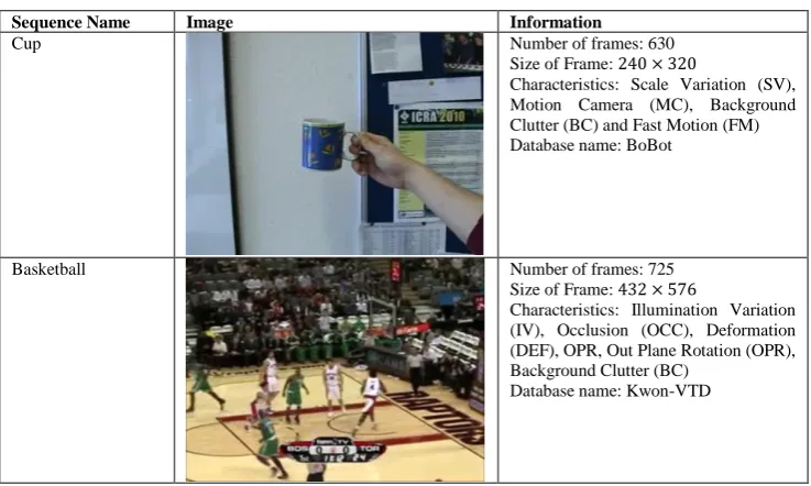
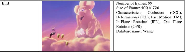
TABLE 6 CHARACTERISTICS OF DATASETS
Sequence Name Image Information
Cup Number of frames: 630
Size of Frame: 240 × 320
Characteristics: Scale Variation (SV), Motion Camera (MC), Background Clutter (BC) and Fast Motion (FM) Database name: BoBot
Basketball Number of frames: 725
Size of Frame: 432 × 576
Characteristics: Illumination Variation (IV), Occlusion (OCC), Deformation (DEF), OPR, Out Plane Rotation (OPR), Background Clutter (BC)
Bird Number of frames: 99 Size of Frame: 400 × 720
Characteristics: Occlusion (OCC), Deformation (DEF), Fast Motion (FM), In-Plane Rotation (IPR), Out Plane Rotation (OPR)
Database name: Wang
TABLE 7 COMPARISON RESULT OF THE PRECISION, RECALL AND F-SCORE FOR CUP, BASKETBALL AND BIRD-2 DATASETS
Metrics MTT KMS DFT SOAMST UIDP BNTP
Cup Precision 0.48 0.63 0.8 0.93 0.945 0.96
Recall 0.4 0.52 0.7 0.87 0.9 0.93
F-Score 0.44 0.57 0.75 0.9 0.92 0.944
Basketball Precision 0.68 0.5 0.6 0.8 0.97 0.98
Recall 0.6 0.36 0.5 0.73 0.91 0.92
F-Score 0.64 0.42 0.55 0.76 0.94 0.95
Bird-2 Precision 0.72 0.64 0.68 0.81 0.95 0.95
Recall 0.66 0.55 0.62 0.73 0.83 0.87
Figure.4 Precision, recall and F-score plots of the proposed BNTP and existing approaches for the cup, basketball, and bird2 datasets
Tracking results
Figure.5 shows the tracking results of our proposed approach on the cup and David. From the figure, we observe that the proposed approach yields better tracking performance in frame 2, frame 35, frame 75 and frame 99.
Frame 2 Frame 35 Frame 75 Frame 99
Figure.5 Tracking results of our proposed approach on the cup and David in different frames
CONCLUSION AND FUTURE WORK
This paper presented a visual tracking approach based on the background normalization and texture pattern analysis. The MWCP algorithm performed clustering of the regions having same intensities and patterns corresponding to the target. The clustering regions are considered as foreground and the remaining irrelevant regions are considered as background. Due to the background normalization, the uneven background is removed. In our proposed work, the patterns are used for the target matching analysis. The classifier determines the likelihood of the extracted patterns and target patterns. Hence, our proposed approach achieves better tracking performance even during the variations in the background and illumination intensity. The proposed approach is compared with the DeepTrack approaches, BMVC, ACCV, TPGR tracker, UIDP, SOAMST, MTT, KMS and DFT. From the comparative analysis, we conclude that the proposed approach achieves higher precision and success rate than the DeepTrack approaches. The proposed BNTP achieves higher average accuracy than the TPGR and DeepTrack trackers. The proposed BNTP approach achieves better precision, recall and F-score performance than the existing approaches. In future, we can present this type of video segmentation system to predict the abnormal activities of the targeted person.
REFERENCES
1. Hong Z, Mei X, Prokhorov D, Tao D, editors. Tracking via robust multi-task multi-view joint sparse representation. Proceedings of the IEEE International Conference on Computer Vision; 2013.
2. Liu B, Huang J, Kulikowski C, Yang L. Robust visual tracking using local sparse appearance model and k-selection. IEEE transactions on pattern analysis and machine intelligence. 2013;35(12):2968-81.
3. Bao C, Wu Y, Ling H, Ji H, editors. Real time robust l1 tracker using accelerated proximal gradient approach. IEEE Conference on Computer Vision and Pattern Recognition (CVPR),; 2012: IEEE.
4. Jia X, Lu H, Yang M-H, editors. Visual tracking via adaptive structural local sparse appearance model. IEEE Conference on Computer vision and pattern recognition (CVPR); 2012: IEEE. 5. Kristan M, Matas J, Leonardis A, Vojir T, Pflugfelder R, Fernandez G, et al. A novel performance evaluation methodology for single-target trackers. 2015.
7. García J, Gardel A, Bravo I, Lázaro JL, Martínez M, Rodríguez D. Directional people counter based on head tracking. IEEE Transactions on Industrial Electronics. 2013;60(9):3991-4000. 8. Du G, Zhang P. A markerless human–robot interface using particle filter and kalman filter for dual robots. IEEE Transactions on Industrial Electronics. 2015;62(4):2257-64.
9. Gao C, Chen F, Yu J-G, Huang R, Sang N. Robust Visual Tracking Using Exemplar-based Detectors. 2015.
10. Zhang Y, Xian B, Ma S. Continuous robust tracking control for magnetic levitation system with unidirectional input constraint. IEEE Transactions on Industrial Electronics. 2015;62(9):5971-80.
11. Ruderman M. Tracking control of motor drives using feedforward friction observer. IEEE Transactions on Industrial Electronics. 2014;61(7):3727-35.
12. Zhao B, Xian B, Zhang Y, Zhang X. Nonlinear robust adaptive tracking control of a quadrotor UAV via immersion and invariance methodology. IEEE Transactions on Industrial Electronics. 2015;62(5):2891-902.
13. Zhang K, Liu Q, Wu Y, Yang M-H. Robust Visual Tracking via Convolutional Networks Without Training. IEEE Transactions on Image Processing. 2016;25(4):1779-92. 14. Pérez P, Hue C, Vermaak J, Gangnet M, editors. Color-based probabilistic tracking. European Conference on Computer Vision; 2002: Springer.
15. Collins RT, Liu Y, Leordeanu M. Online selection of discriminative tracking features. IEEE transactions on pattern analysis and machine intelligence. 2005;27(10):1631-43. 16. Adam A, Rivlin E, Shimshoni I, editors. Robust fragments-based tracking using the integral histogram. 2006 IEEE Computer Society Conference on Computer Vision and Pattern Recognition (CVPR'06); 2006: IEEE.
17. Hare S, Saffari A, Torr PH, editors. Struck: Structured output tracking with kernels. 2011 International Conference on Computer Vision; 2011: IEEE.
18. Yang F, Lu H, Yang M-H. Robust superpixel tracking. IEEE Transactions on Image Processing. 2014;23(4):1639-51. 19. Henriques JF, Caseiro R, Martins P, Batista J. High-speed tracking with kernelized correlation filters. IEEE Transactions on Pattern Analysis and Machine Intelligence. 2015;37(3):583-96. 20. Ma B, Shen J, Liu Y, Hu H, Shao L, Li X. Visual tracking using strong classifier and structural local sparse descriptors. IEEE Transactions on Multimedia. 2015;17(10):1818-28. 21. Kalal Z, Matas J, Mikolajczyk K, editors. Pn learning: Bootstrapping binary classifiers by structural constraints. IEEE Conference on Computer Vision and Pattern Recognition (CVPR); 2010: IEEE.
22. Zhang K, Zhang L, Yang M-H. Fast compressive tracking. IEEE Transactions on Pattern Analysis and Machine Intelligence. 2014;36(10):2002-15.
23. Song H. Robust visual tracking via online informative feature selection. Electronics Letters. 2014;50(25):1931-3.
24. Yu Z, Deng Y, Jain AK, editors. Keystroke dynamics for user authentication. IEEE Computer Society Conference on Computer Vision and Pattern Recognition Workshops (CVPRW), 2012 2012 16-21 June 2012.
25. Gao J, Ling H, Hu W, Xing J, editors. Transfer learning based visual tracking with gaussian processes regression. European Conference on Computer Vision; 2014: Springer.
26. Nanni L, Lumini A, Brahnam S. Survey on LBP based texture descriptors for image classification. Expert Systems with Applications. 2012;39(3):3634-41.
27. Ojala T, Pietikainen M, Maenpaa T. Multiresolution gray-scale and rotation invariant texture classification with local binary patterns. IEEE Transactions on pattern analysis and machine intelligence. 2002;24(7):971-87.
28. Ning J, Zhang L, Zhang D, Wu C. Robust object tracking using joint color-texture histogram. International Journal of
Pattern Recognition and Artificial Intelligence. 2009;23(07):1245-63.
29. Subrahmanyam M, Maheshwari R, Balasubramanian R. Local maximum edge binary patterns: a new descriptor for image retrieval and object tracking. Signal Processing. 2012;92(6):1467-79.
30. Babaee M, You Y, Rigoll G. Combined segmentation, reconstruction, and tracking of multiple targets in multi-view video sequences. Computer Vision and Image Understanding. 2016.
31. Wang X, Gao B, Masnou S, Chen L, Theurkauff I, Cottin-Bizonne C, et al. Active colloids segmentation and tracking. Pattern Recognition. 2016;60:177-88.
32. Liwicki S, Zafeiriou SP, Pantic M. Online kernel slow feature analysis for temporal video segmentation and tracking. IEEE transactions on image processing. 2015;24(10):2955-70. 33. Xiaojun W, Feng P, Eeihong W. Tracking of moving target based on video motion nuclear algorithm. International Journal on Smart Sensing and Intelligent Systems. 2015;8(1):181-98. 34. Drayer B, Brox T. Object Detection, Tracking, and Motion Segmentation for Object-level Video Segmentation. arXiv preprint arXiv:160803066. 2016.
35. Khoreva A, Benenson R, Galasso F, Hein M, Schiele B. Improved Image Boundaries for Better Video Segmentation. arXiv preprint arXiv:160503718. 2016.
36. Keuper M, Brox T. Point-wise mutual information-based video segmentation with high temporal consistency. arXiv preprint arXiv:160602467. 2016.
37. Spina TV, Falcão AX. FOMTrace: Interactive Video Segmentation By Image Graphs and Fuzzy Object Models. arXiv preprint arXiv:160603369. 2016.
38. Jiang H, Zhang G, Wang H, Bao H. Spatio-temporal video segmentation of static scenes and its applications. IEEE Transactions on Multimedia. 2015;17(1):3-15.
39. Li C, Lin L, Zuo W, Wang W, Tang J. An Approach to Streaming Video Segmentation With Sub-Optimal Low-Rank Decomposition. IEEE Transactions on Image Processing. 2016;25(5):1947-60.
40. Chen L, Shen J, Wang W, Ni B. Video object segmentation via dense trajectories. IEEE Transactions on Multimedia. 2015;17(12):2225-34.
41. Delibasis KK, Goudas T, Maglogiannis I. A novel robust approach for handling illumination changes in video segmentation. Engineering Applications of Artificial Intelligence. 2016;49:43-60.
42. Gangapure VN, Nanda S, Chowdhury AS, Jiang X, editors. Causal video segmentation using superseeds and graph matching. International Workshop on Graph-Based Representations in Pattern Recognition; 2015: Springer.
43. Wang H, Raiko T, Lensu L, Wang T, Karhunen J. Semi-Supervised Domain Adaptation for Weakly Labeled Semantic Video Object Segmentation. arXiv preprint arXiv:160602280. 2016.
44. Abdelwahab MA, Abdelwahab MM, Uchiyama H, Shimada A, Taniguchi R-i, editors. Video Object Segmentation Based on Superpixel Trajectories. International Conference Image Analysis and Recognition; 2016: Springer.
45. Husain F, Dellen B, Torras C. Consistent depth video segmentation using adaptive surface models. IEEE transactions on cybernetics. 2015;45(2):266-78.
46. Molina-Giraldo S, Carvajal-González J, Álvarez-Meza A, Castellanos-Domínguez G. Video segmentation framework based on multi-kernel representations and feature relevance analysis for object classification. Pattern Recognition Applications and Methods: Springer; 2015. p. 273-83.
48. Razavi SF, Sajedi H, Shiri ME. Integration of colour and uniform interlaced derivative patterns for object tracking. IET Image Processing. 2016;10(5):381-90.
49. VOT 2013 dataset 2017. Available from: http://votchallenge. net/vot2013/dataset.html.
50. Visual Tracker Benchmark. Available from: http://visual-tracking.net.
51. Bonn Uo. [cited 2016 21.09.2016]. Available from: http://iai.uni-bonn.de/~kleind/tracking.
52. Visual Object Tracking (VOT) 2013 Benchmark 2013 [cited 2016 21.09.2016]. Available from: http://votchallenge.net /vot2013/results.html.
53. Li H, Li Y, Porikli F. DeepTrack: Learning discriminative feature representations by convolutional neural networks for visual tracking. Proc, BMVC. 2014:1-12.
54. Ning J, Zhang L, Zhang D, Wu C. Scale and orientation adaptive mean shift tracking. IET Computer Vision. 2012;6(1):52-61.
55. Zhang T, Ghanem B, Liu S, Ahuja N, editors. Robust visual tracking via multi-task sparse learning. IEEE Conference on Computer Vision and Pattern Recognition (CVPR); 2012: IEEE. 56. Li X, Zhang T, Shen X, Sun J. Object tracking using an adaptive Kalman filter combined with mean shift. Optical Engineering. 2010;49(2):020503--3.
57. Sevilla-Lara L, Learned-Miller E, editors. Distribution fields for tracking. IEEE Conference on Computer Vision and Pattern Recognition (CVPR); 2012: IEEE.
58. Beyan C, Temizel A. Adaptive mean-shift for automated multi object tracking. IET computer vision. 2012;6(1):1-12.
Cite this article as:
V.Rajagopal and B.Sankaragomathi. Background normalization and texture pattern-based video segmentation for visual tracking. Int. Res. J. Pharm. 2017;8(11):184-195 http://dx.doi.org/ 10.7897/2230-8407.0811239
Source of support: Nil, Conflict of interest: None Declared