Characteristics of the pipe junction with 2.4 cross-section area ratio for
the case of the flow division
J. Štigler1a and O. Šperka1
1
Brno University of Technology, Faculty of Mechanical Engineering, Energy Institute, Victor Kaplan Department of Fluid Engineering, Technická 2896/2, 616 69, Czech Republic
Abstract. There are presented characteristics of the pipe junction for the case of the flow division in this paper. The pipe junction consists of one straight pipe, with the diameter 50 mm and one adjacent pipe with diameter 32 mm. The characteristics have been measured for five different angles of the adjacent pipe.
1 Introduction
aMany papers, about the fluid flow in the pipe junction, have been written by these authors. It is possible to use it for the fluid flow solution in the pipe line net. There are some other mathematical models but they are based on the unrealistic assumptions or their coefficients have not any physical meaning. [1, 2] The new mathematical model for the 90° pipe junction together with its coefficients is described in [3, 4]. The improved mathematical model for the arbitrary angle of the adjacent branch is introduced in the [5]. Some discussion about mathematical model for the unsteady fluid flow in pipe junction has been presented in [6]. A lot of numerical solutions and experiments of the fluid flow in the pipe junction have been done in past few years. For example numerical study of fluid flow has been presented in the [7, 8]. The PIV measurement of the fluid flow in the pipe junction has been described in [9] The Comparison of the PIV measurement with numerical solution of fluid flow in [10]. The first new characteristics obtained by measuring and its comparison with CFD calculations were presented at [11]. Many papers have been written about fluid flow in pipe junction as it was mentioned above and reader can get most of them on the internet. This paper will be therefore dedicated mainly to the presentation of the coefficients obtained by measurements. And more over the discussion about the results will be included in this paper.
2 Mathematical model
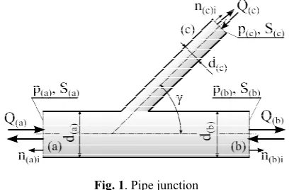
The pipe junction it is dealt with is drawn in the figure 1.
a
The mathematical model of the fluid flow in the pipe junction consists of three equations which describe the relationship between the flow rates and pressures at the border of the pipe junction area.
Fig. 1. Pipe junction
The border of the pipe junction area is delimited by the cross-sections S(a), S(b) and S(c) placed in such distance
from the flow division domain where the flow is not disturbed by the pipe junction. The minimum distance to ensure this assumption is about 10 diameters at each branch.
First equation of the mathematical model of the pipe junction is the power equation. This equation represents the mechanical energy conservation law in the pipe junction
0 2
1 2
2 2
2 2
2 2
2 2
2 2
) mX ( ) X (
) mX ( ) P ( ) mc ( ) c ( ) c (
) mc (
) mb ( ) b ( ) b (
) mb ( ) ma ( ) a ( ) a (
) ma (
Q S . Q Q
p S Q
Q p S Q Q
p S Q
. (1)
The second equation is the momentum equation. This is a vector equation but we will take into consideration only
This is an Open Access article distributed under the terms of the Creative Commons Attribution License 2 0 , which . permits unrestricted use, distributi and reproduction in any medium, provided the original work is properly cited.
on,
C
the component in the direction of branch “b” this direction is represented by the unit normal vector n(b)i.
This is clear from the figure 1
0 2 2 2 2 ) X ( ) mX ( i ) M ( i ) c ( ) c ( ) c ( ) c ( ) mc ( i ) b ( ) b ( ) b ( ) b ( ) mb ( i ) a ( ) a ( ) a ( ) a ( ) ma ( S Q n S p S Q n S p S Q n S p S Q . (2)
This equation has to be multiplied by the vector n(b)i to
get the component equation in that direction. The last third equation is continuity equation
0
(mb) (mc) )
ma
( Q Q
Q
. (3)
The summation convection is used in the above equations. This mathematical model is valid under these assumptions
Steady fluid flow
The gravity vector is perpendicular to the pipe junction plain.
The density is constant
The Coriolis numbers and Bousineques numbers on the cross-sections S(a), S(b), and S(c)
are equal to 1.
It is possible to remove all these assumptions in the general mathematical model [5 ].
The index “X” in the above equations has to be replaced by the index “a”, “b” or “c”. It depends on branch to which the coefficients (M)i and (P) will be related to.
3 Pipe junction coefficients
Two coefficients appear in the mathematical model. The power coefficient (P) can be expressed from the equation
(1). This coefficient represents the energy losses in the pipe junction. It is proportional to the kinetic energy per time in one of the branches for which the coefficient will be derived.
The momentum coefficient (M)i can be expressed from
the equation (2). This coefficient is proportional to the force which the fluid impacts on the pipe junction. The total force can be obtained by multiplying of this coefficient with the total momentum of fluid in branch for which the coefficient was derived. In this case we will take into consideration the component of this coefficient only in the direction of branch “b”.
The momentum coefficient depends also on the total pressure at all branches. If all parameters as shape of pipe junction, flow configuration, flow rates, differences of pressures between the branches are the same then the coefficients varies with total pressure. Therefore it is necessary to relates all pressures to the constant value pressure in some branch. In case of this paper the pressure value in branch “a” is taken as zero. It means that the momentum coefficient is derived for case zero
pressure level in branch “a”. It means that the momentum coefficient will be expressed from this modified momentum equation 0 2 2 2 2 ) X ( ) mX ( i ) M ( i ) c ( ) c ( ) ca ( ) c ( ) mc ( i ) b ( ) b ( ) ba ( ) b ( ) mb ( i ) a ( ) a ( ) ma ( S Q n S p S Q n S p S Q n S Q . (4) Where ) a ( ) b ( ) ba
( p p
p
(5) and ) a ( ) c ( ) ca
( p p
p
. (6)
Now the unknowns are three mass flow rates Q(ma), Q(mb)
and Q(mc) and absolute pressure p(a) and two pressure
differences p(ba) and p(ca) instead of three absolute
pressures p(a), p(b) and p(c).
Both coefficients can be divided into two parts. First parts will be related to the friction losses in the pipe junction. They will be called friction coefficients. Second parts will be related to the shape of pipe junction. They will be called geometry coefficients. It can be expressed this way
) PG ( ) PF ( ) P (
(7)
and i ) MG ( i ) MF ( i ) M ( . (8)
The total coefficients can be obtained by the measurements. The friction coefficients can be obtained from the known friction losses, represented by the pressure drop, in straight pipes. The friction power coefficient can be expressed as follow
) mX ( ) mX ( ) X ( ) c ( ) c ( ) c ( ) b ( ) b ( ) b ( ) a ( ) a ( ) a ( ) PF ( Q Q S L Q i L Q i L Q i 2 2 2 2 . (9)The friction momentum coefficient can be expressed as follow
2 ) mX ( ) X ( i ) c ( ) c ( ) c ( ) c ( i ) b ( ) b ( ) b ( ) b ( i ) a ( ) a ( ) a ( ) a ( i ) MF ( Q S n S L i n S L i n S L i . (10)The component of friction momentum coefficient in direction branch “b” will be obtained by multiplying previous equation with unit normal vector n(b)i.
The quantities i(a), i(b), and i(c) are pressure drops in the
branches “a”, “b” and “c” with flow rates Q(a), Q(b) and
Q(c) without pipe junction influence.
The geometry coefficients can be then evaluated from the expressions (11) and (12)
) PF ( ) P ( ) PG (
(11)
i ) MF ( i ) M ( i ) MG
(
. (12)
Advantages of the geometry coefficients are
They are independent on the total flow rate in the pipe junction
They are the same for the all geometrically similar pipe junctions
But it is necessary to remember that these coefficients depend on the flow configuration in the pipe junction and on the flow rate ratio between two branches. In case of flow divisions the three flow configurations are possible. It is apparent from a figure 2.
“Div a”, (Da) “Div b”, (Db) “Div c”, (Dc) Fig. 2. Flow configuration for the flow division.
It is necessary to know the function for momentum geometry coefficient and the function for power geometry coefficient. It means it is necessary to know two functions or characteristics for each flow configuration.
4 Experiment description
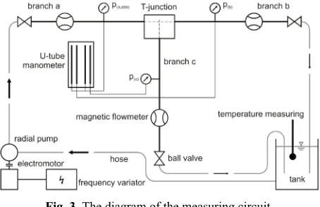
The testing circuit was built in the Victor Kaplan’s Department of Fluid Engineering laboratory. The pipe junction was drilled in plastic blocks. It ensured the sharp edges at the division domain. Five pipe junctions, each for the different angle of the adjacent branch, were measured. The angles of the adjacent branch were 30°, 45°, 60°, 75°, 90°. The gauged parameters was as follows Flow rates at each branch gauged by the magnetic flow meters, absolute pressure gauged by the pressure transducer, pressure differences between branches “b”-“a” and “c”-“b”-“a”, pressure differences was gauged both by differential pressure manometer and also by U-tube manometer. It is necessary to say that for the characteristics evaluation the values from the U-tube manometer were used. The last gauged parameter was water temperature.
Fig. 3. The diagram of the measuring circuit.
The diagram of the test circuit is drawn in the figure 3. The flow rate was controlled by pump equipped by the
frequency converter and by the valves placed at each branch.
The fluid flow in some flow configurations was unstable therefore all parameters were gauged three times. Eleven flow rate ratios were measured for each flow configuration. Each configuration for all flow rate ratios was measured twice to ensure that the results are correct. There is a picture of testing circle in the figure 4 and the picture of PIV measurements at the figure 5.
Fig. 4. The test circuit for the pipe junction characteristics measuring.
Fig. 5. The picture of the PIV measuring.
5 Characteristics of pipe junction
The resultant characteristics will be presented in this chapter. The characteristics for nine different angles will be drawn in the charts. The characteristics for the angles bigger than 90° are recalculated from the characteristics for the angles less than 90°.
.
5.1. Flow configuration “Div a”
The coefficients (PG) and (MG)1 are drawn as a function
of flow rate ratio q(ca) in the figure 4 and 5
) a (
) c ( ) ca (
Q Q q
.
(13)
There are some interesting results. It is apparent, from the figure 6, that lowest losses are for low values q(ca) for
angle 30°, for the middle values of q(ca) are lowest losses
angle 60°. The interesting result is that the losses are not lowest for whole range of q(ca) for pipe junction with
angle 30°.
In case of momentum coefficient it is interesting, that the coefficients for the angles 30° and 150°, 45° and 135°, 60° and 120°, 75° and 105° are rather close to each other and the maximal values are for the angle 90°.
Fig. 6. The (PG) coefficients for flow configuration “Div a” as a
function of flow rate ratio q(ca).
Fig. 7. The (MG)i coefficients for flow configuration “Div a” as
a function of flow rate ratio q(ca).
One will expect that the biggest momentum coefficient will be for the angle 150°. But this phenomenon can be explained this way. In case of the angle 150° the pressure in branch “b”, for big values of q(ca), increases a lot. This
pressure acts against force caused by the flow direction change. Therefore the resulting force is less than the force for the angle 90°.
5.2. Flow configuration “Div b”
The comments of this case are almost identical to the the comments in case of flow configuration Div a. The variable for the pipe junction coefficients evaluation is flow rate ratio q(cb) in this case
) b (
) c ( ) cb (
Q Q q
.
(14)
The power geometry coefficient is identical to the one for the flow configuration Div a.
In case of momentum geometry coefficient one will expect that the curves for the flow configuration “Div a” and angle 30° will be symmetrical about zero value with the flow configuration “Div b” angle 150° and similarly
for the other pairs of the angles. But this is not true. It is caused by the reference zero pressure in branch “a”. It would be symmetrical in case when all pressures will be related to the zero pressure p(b) in case of flow
configuration “Div b”. This is the case where it is possible to see the influence of the absolute pressure in branches.
Fig. 8. The (PG) coefficients for flow configuration “Div b” as a
function of flow rate ratio q(ca).
Fig. 9. The (MG)i coefficients for flow configuration “Div b” as
a function of flow rate ratio q(ca).
5.3. Flow configuration “Div c”
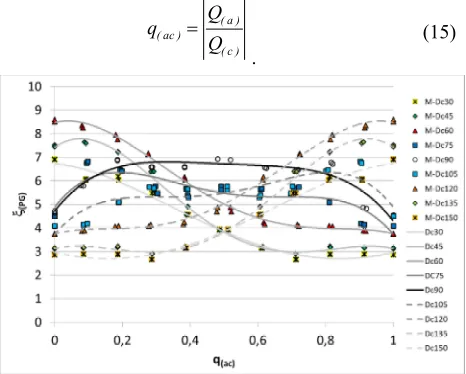
The variable for the pipe junction coefficients evaluation is flow rate ratio q(ac) in this case
) c (
) a ( ) ac (
Q Q q
.
(15)
Fig. 10. The (PG) coefficients for flow configuration “Div c” as
The results for the power geometry coefficient look rather reasonable.
Fig. 11. The (MG)i coefficients for flow configuration “Div c”
as a function of flow rate ratio q(ca).
This flow configuration was very difficult to measure, because the flow was very unstable for the high values of
q(ac).
The curves for the pairs of the angles (30°-150°, 45°-135° and so on) are not symmetrical about the zero value of momentum coefficient. The reason is the same as in the case of flow configuration “Div a” and “Div b”.
6 Characteristics of pipe junction as a polynomial functions
Characteristics of the pipe junction as a polynomial functions will be presented in this chapter. The polynomial functions were drawn to approximate the measured values. The general form of the polynomial function is as follow
N
i i
) xy ( iq
A 0
.
(16)
The quantity q(xy) is the flow rate ratio related to the
particular flow configuration.
Table 1. Polynom coefficients for the coefficient (PG) for the
flow combination “Div a”. Variable is q(ca)
Agl. A(0) A(1) A(2) A(3) A(4)
30° 0.03996 0.21542 - 1.98045 5.96808 45° 0.00494 0.69511 - 2.64166 5.30444 60° - 0.03018 0.87583 - 2.18938 4.62091 75° - 0.02644 0.54269 0.22227 2.77669 90° - 0.01502 0.72022 - 0.50585 3.34952 105° - 0.04975 0.13346 2.99545 2.13002 120° - 0.04764 - 0.11965 4.90077 1.62379 135° - 0.05694 0.02440 5.34726 2.24393 150° - 0.04610 0.77084 3.13437 5.61312
Table 2. Polynom coefficients for the coefficient (MG)1 for the
flow combination Diva. Variable is q(ca)
Agl. A(0) A(1) A(2) A(3) A(4)
30° 0.06386 - 0.03327 0.50067 -0.30472 45° 0.04349 0.30411 0.01003 -0.17258 60° 0.01982 0.52247 - 0.15851 -0.07909 75° 0.00073 0.67438 0.13419 -0.31179 90° - 0.01433 0.77718 0.18345 -0.27213 105° - 0.04652 0.78045 0.14711 -0.15718 120° - 0.06140 0.90204 - 0.22418 0.08071 135° - 0.07597 0.92531 - 0.75895 0.43393 150° - 0.06522 0.59853 - 0.65970 0.26504
Table 3. Polynom coefficients for the coefficient (PG) for the
flow combination “Div b”. Variable is q(cb)
Agl. A(0) A(1) A(2) A(3) A(4)
30° - 0.04610 0.77084 3.13437 5.61312 45° - 0.05694 0.02440 5.34726 2.24393 60° - 0.04764 - 0.11965 4.90077 1.62379 75° - 0.04975 0.13346 2.99545 2.13002 90° - 0.01502 0.72022 - 0.50585 3.34952 105° - 0.02644 0.54269 0.22227 2.77669 120° - 0.03018 0.87583 2.18938 4.62091 135° 0.00494 0.69511 - 2.64166 5.30444 150° 0.03996 0.21542 - 1.98045 5.96808
Table 4. Polynom coefficients for the coefficient (MG)1 for the
flow combination “Div b”. Variable is q(cb)
Ang. A(0) A(1) A(2) A(3) A(4)
30° - 0.02744 - 0.15783 0.48191 -0.35726 45° 0.00565 - 0.55647 0.51469 -0.42874 60° 0.01008 - 0.61420 - 0.02193 -0.03182 75° 0.01988 - 0.62134 - 0.28020 0.18022 90° 0.01433 - 0.77718 - 0.18345 0.27213 105° 0.02839 - 0.83435 0.00595 0.28218 120° 0.03744 - 0.83957 0.41874 0.03667 135° 0.04040 - 0.73097 0.34852 0.10066 150° 0.04242 - 0.49984 - 0.07477 0.23415
Table 5. Polynom coefficients for the coefficient (PG) for the
flow combination “Div c”. Variable is q(ac)
Ang. A(0) A(1) A(2) A(3) A(4)
30° 6.7239 1.10915 - 19.578 24.26525 -7.34314 45° 7.4166 10.5006 - 81.598 118.1849 -51.384 60° 8.475 3.53416 - 49.05 71.86643 -31.063 75° 4.8848 18.66 - 76.133 108.396 -52.067 90° 4.7174 18.2622 - 57.23 76.319 -37.769 105° 3.7407 16.6857 -63.345 99.87026 -52.067 120° 3.76249 3.21864 - 19.829 52.38555 -31.063 135° 3.12062 3.67499 - 35.345 87.34959 -51.384 150° 2.95850 - 3.1574 9.15858 5.10732 -7.3431
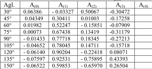
Table 6. Polynom coefficients for the coefficient (MG)1 for the
flow combination “Div c”. Variable is q(ac)
Ang A(0) A(1) A(2) A(3) A(4)
30° 0.45341 - 1.165 2.17698 1.82076 -2.9947 45° 0.05468 - 2.706 13.51148 - 17.397 6.70083 60° - 0.184 - 0.857 7.98778 - 12.606 5.75276 75° 0.00097 - 0.2549 0.33661 -0.02042
90° - 0.0566 0.07725 0.03645 105° - 0.1144 0.59046 -0.30261
120° - 0.0394 - 0.6178 2.42304 -1.10727
135° - 0.0125 - 0.1635 - 2.57935 10.44418 -6.9974 150° 0.04895 - 1.9576 7.45342 - 6.42768 1.49592
7 Conclusion
The characteristics of the pipe junction for flow division with the five different angles of the adjacent branch were presented in this article. All characteristics were derived calculated under the next assumptions
Steady fluid flow
The gravity vector is perpendicular to the pipe junction plain.
The density is constant
The Coriolis numbers and Bousineques numbers on the cross-sections S(a), S(b), and S(c)
The reference pressure is p(a)=0
The discussion about the pipe junction coefficients and their explanation was also included in this paper. The interesting results was obtained for the minimum hydraulic losses for flow configuration “Div a” and “Div b”. The coefficients of polynomial functions for all measured characteristics were listed at the end of the paper.
8 Acknowledgement
The authors are grateful to the Grant Agency of Czech Republic (GACR) for funding this research under project “Mathematical and Numerical Modeling of Flow in Pipe Junction and its Comparison with Experiment”. Registration number of this project is 101/09/1539.
9 References
1. D. S. Miller, Internal flow, A guide to losses in pipe and duct systems,
2. K. Oka, H. Ito. J Fluid Eng. 127, 110, (2005) 3. J. Štigler, J. Mech. Eng. 5,249-262, (2006) 4. J. Štigler, J. Mech. Eng. 5,263-270, (2006)
5. J. Štigler, IOP Conf. Ser.:Earth Environ. Sci., 12, 12101, (2010)
6. J. Štigler, Scientific Buletin of the “Politechnica” University of Timisoara, Romania Transactions on Mechanics, 6, 83-92, (2007)
7. L. Beneš, P. Louda, R. Keslerová, J. Štigler, J. Amc., 04,074, (2011), (In press)
8. P. Louda, K. Kozel, J. Příhoda, L. Benes, J. Compfluid., 12, 003, (2010)
9. M. Kotek, V. Kopecký, D. Jašíková, Recent Researches in Mechanics, Proc. of the 2nd International Conference on Fluid Mechanics and Heat and Mass Transfer 2011 (FLUIDSHEAT11) WSEAS Cofru,169-172,(2011)
10. J. Štigler, R. Klas, M. Kotek, V. Kopecký, J. Proeng., 39, 19-27, (2012)