Automatic Segmentation of Fiber Cross
Sections by Dual Thresholding
Yan Wan1,Li Yao1,Bugao Xu2
1
Donghua University, School of Computer Science, Shanghai, Shanghai CHINA
2
University of Texas, Human Ecology, Austin, TX UNITED STATES
Correspondence to:
Bugao Xu email: [email protected]
ABSTRACT
In a microscopic image, fiber cross sections are often surrounded by borders distinctively darker than their bodies and the background. Fiber borders can be utilized to separate cross-sections properly so that accurate fiber shape and size information can be obtained. Hence, locating correct fiber borders is one of the most critical steps in cross-sectional analysis for fiber characterization and identification. This paper introduces a dual-thresholding algorithm that performs automatic fiber border segmentation from noisy cross-sectional images. The dual thresholds include a low threshold calculated based on the histogram of the difference from the average grayscale, and a high threshold computed by a bisection algorithm. With the low threshold, part of fiber border pixels, regarded as seeds, can be reliably located. The seeds can be further expanded by using the high threshold to form complete borders surrounding individual cross-sections. The experimental results show that the dual-thresholding algorithm can obtain cleaner and more fiber borders than other connectional thresholding algorithms, and improves the detection accuracy from 52.78% and 88.88%.
INTRODUCTION
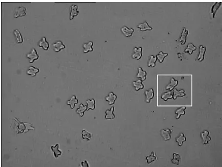
Fiber characterization and identification are often performed on fiber cross-sectional images, which possess inherent information about fiber geometrical features [1-10]. Fiber identification methods using image-processing techniques generally take five steps: sample preparation, image capturing, fiber detection and segmentation, shape analysis, and fiber classification. In sample preparation, a bundle of fibers is often embedded in a polymer resin, hardened and cut into slices of 1-4 m in thickness [11][12]. The slices are then placed on a slide, and the embedding resin is removed by dissolving solvent. Crossed-sectional image are taken under a microscope. Figure 1 shows a cross-sectional image of cross-shaped fibers captured by a Nikon Eclipse
50i microscope coupled with a CCD camera. The picture is 640×480 in pixels. It can be observed that fibers are surrounded by darker borders, which are probably due to refractive light on the interface between fiber edges and air. The darkness and width of dark borders can vary with the thickness of a fiber slice, but the areas (fiber bodies) encompassed by borders seem less changeable.
As demonstrated in the previous work [6-10], fiber segmentation appears to be the most important function in an automatic fiber-image-analysis system for achieving accurate cross-section measurements, because the segmentation dictates the information of final fiber contours and thus feature measurements needed for classifications. Although the fiber borders vary in brightness and thickness, the circumscribed areas are the fiber bodies. Therefore, detecting these borders provides a reliable way to segment fiber cross-sections from the intricate background.
FIGURE 1. Fiber cross-section image from Nikon 50i light microscope system.
Table I lists some of the conventional edge detectors and their effects on locating fiber cross-sections. It can be seen that these edge-detection methods tend to generate pseudo, dual and/or broken edges when the image is noisy, unevenly illuminated or defocused, so the completed fiber with closed and accurate border is hard to be obtained, which would lead to false measurements and identification. A single-pixel contour also increases ambiguity of separating overlapped fibers [9].
TABLE I. Fiber contours detected by conventional edge detectors.
Various thresh holding techniques have been also used to extract fiber borders [13], [14]. Global thresholding selects a single threshold from the histogram of the entire image, while local thresholding uses localized grayscale information to calculate adaptive thresholds across the image. Global thresholding is simple to implement but is likely to produce biased results when the illumination is not uniform. Local thresholding methods can deal with non-uniform illumination but they are more sensitive to localized noise.
In this paper, we present a dual-thresholding algorithm that combines the features of both global and local thresholding to extract accurate and complete fiber boundaries, and the fiber segmentation results in comparison with other conventional algorithms. The proposed algorithm is specifically designed to handle typical microscopic images captured by a similar imaging system to the one used in this research, and fibers that has on average 20-µm diameter. We will use a partial image of Figure 1.
(marked by a rectangle in the image) as an example for explaining the algorithm in the discussion.
DUALTHRESHOLDING
Since the intensity of a fiber image can be easily affected by the illumination and the thickness of the slice, the grayscales of pixels are not reliable information for image thresholding. The proposed dual-thresholding algorithm is based on the contrasts, i.e., the difference from the mean grayscales, of pixels. Let (i, j) be the pixel in the ith row and the jth column in a fiber image I with width U and height V, Ii,j is the
grayscale of pixel (i, j), and the arithmetic average, M(i,j), of the grayscales of pixels in a w×h window centered at (i, j) be Ai,j. Then
s j i M l k
l k
j i
M I A
( ,) (,)
,
, (1)
where Ms is the cardinality of M(i,j), which can be
denoted as the area of the rectangle window:
h
w
M
s
(2)where w=min(2×i, w, 2×|U-i|), h=min(2×j, h, 2× |V-j|). The difference from the average grayscale at pixel (i, j) is:
) ( , ,
,j ij ij
i I A
D (3)
FIGURE 2. The distribution of D of the fiber image.
Low Threshold
The low threshold l is a global threshold used to locate part of dark pixel for each fiber border. Firstly, use the average grayscale of the image as an initial threshold to roughly segment fiber border pixels, which are called set B. Equally divide B into K zones, and count the pixels in each zone to calculate the corresponding D histogram. Figure 3 displays the two D histograms for the image in Figure 1 when K=20 and K=500, respectively. Both histograms show a similar shape in which a peak (i.e., the highest point) falls in a range of (-10000, -5000).
FIGURE 3. D histograms ofpixels.
The location of the peak can be approximately determined in a simple way. First, locate the peak, P1, on the histogram of the smaller K. Then, smooth the histogram of the larger K with moving averages. Finally, search for the peak P2 on the smoothed histogram that is nearest to P1. The D value corresponding to P2 can be used as the low threshold, l. With l, a set of pixels L can be obtained by using Eq. (4).
i j D l i j I
L (, ) i,j ,(, ) (4)
L should contain some pixels of each fiber border because l corresponds to the most pixels in the image. Figure 4 displays three crossed fibers (a) marked in Figure 1 and the detected fiber borders (b) with l. Due to the variations in thickness, the fiber cross-sections exhibit different grayscales along their borders. As seen in Figure 4b, some border pixels are inevitably missing from L because their D values are higher than l. L is regarded as an initial set in the next step, and therefore the found pixels in L are the seeds that can grow into complete fiber borders when the thresholding condition is lowered.
FIGURE 4. Fiber image (a) and border pixels (b) segmented by using low threshold l
High Threshold
The purpose of selecting a high threshold, h, is to expand the pixels found with the low threshold into complete fiber borders using more lenient criteria while preventing spurious noise—pixels protruding out of fiber borders. As shown in Figure 5, spurious noise can greatly contort the shape of the fiber or create connections with other fiber borders, and thus must be excluded from the final set, H, of pixels representing fiber borders:
i j D h i j I
H (, ) i,j ,(, ) (5)
-3 -2.5 -2 -1.5 -1 -0.5 0
0 100 200 300 400 500 600 700 800 900
D (x104)
K=500
P2
Pixels
Pixe
ls
10
4
-3 -2.5 -2 -1.5 -1 -0.5 0
D (x104)
0 0.5 1 1.5 2.5
2
K=20
FIGURE 5. Spurious noise (pointed by arrows).
The determination of h is an iterative procedure. Let be the difference of the hs calculated in two consecutive iterations, and k the times of iteration. The procedure of finding the final h is terminated when the following condition is satisfied:
k k
l
2 1 2
1
1 (6)
i.e.,
lklog2 (7)
A bisection algorithm is used to determine the high threshold h as follows:
1. Let h be 0.
2. Let ltemp = l, htemp = h, and ltemp < htemp.
3. The error is the difference between ltemp and
htemp. If the algorithm is convergent, i.e. |ltemp-
htemp | < , then the procedure finishes.
Otherwise, go to step 4.
4. Let
2
temp
temp l
h
h . Based on h, set H is obtained:
i j D h i j I
H (, ) i,j ,(, ) (8)
Apparently, L is a subset of , which contains both fiber border pixels and other unwanted pixels (background or noise).
5. Use pixels in L as seeds to recursively search connected pixels in the 3x3 window in H. Once one pixel in the 3x3 window is located, it is marked as a new seed, and the seaching continues until no neighbor pixel is found for all the seeds. The unsearched pixels in H are those islated noise pixels that are simply delected. 6. The saved pixels may contain spurious branches
(Figure 5), which need to be eliminated based on the preset limit on the allowed length of branches. When the number of protruding pixels
is larger than 5, a branch can seriously influencethe shape of a fiber border, and thus, go to step 7 to modify htemp. Otherwise, go to step 8
to modify ltemp.
7. Let htemp = l. Go to step 3.
8. Let ltemp = l. Go to step 3.
In the experiment, it was found that when is less than 50, the difference between two consecutive fiber border sets (H) was inconspicuous, and thus, the process of finding the high threshold h may be terminated. Normally, eight iterations are enough for finding a suitable h.
Figure 6 displays the detected fiber border sets of Figure 4 in the eight iterations of selecting the high threshold. In the first iteration as shown in Figure 6(a), the calculated h was -5000 and not enough pixels were detected to make all the fiber orders complete. In the second iteration, h became too high (-2500) and more noise pixels appeared. In the following iterations, high and low h values alternated, but the difference in detected pixels became smaller. With this bisection method, the final h (-3945) was selected.
(a) h = -5000 (b) h = -2500
(c) h = -3750 (d ) h = -4375
(e) h = -4062 (f) h = -3906
(g) h = -3984 (h) h = -3945
In the dual-thresholding algorithm, the low threshold is used to control isolated noise (small objects) in the image while the high threshold is used to control connective noise (branches connecting fiber borders). As shown in Figure 6(h), some isolated pixel clusters (noise) may be still included in H after the thresholding. These small objects can be removed by using an area threshold since they consist of much smaller numbers of pixels than a fiber border.
Experiment
The borders of various fiber cross sections detected by the dual-thresholding algorithm were compared with those detected by several conventional thresholding algorithms, such as Otsu [16], one-dimensional entropy [17], two-dimensional entropy [18], and minimum error thresholding [19] (see Table II). From the samples, it can be seen that the conventional algorithms exhibit difference performances when applied to process different fibers. Some of them are sensitive to isolate noise (e.g., the One-Dimensional Entropy algorithm for cotton), while others are unable to form complete fiber borders (e.g., the Minimum Error Thresholding algorithm for the trilobal fiber). On the other hand, the dual-thresholding algorithm shows the most consistent outcome for all the processed fibers with clean and complete borders.
TABLE II. Comparison of different thresholding algorithms.
Fiber image
Otsu
1-D
Entropy
2-D
Entropy
Minimum Error
Dual Thresholding
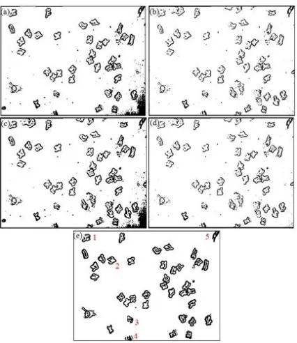
A full image of cross-shaped fibers (Figure 1) was also processed with these algorithms. Figure 7 displays the segmentation results of this image from Otsu, 1-D
entropy, 2-D entropy, minimum error, and the dual-thresholding algorithms. As shown in Figures 7(a) and (c), Otsu and 2-D entropy algorithms were sensitive to non-uniformly illumination in the image, yielding large spots in the lower-right corner, but were unable to seal the borders of many fibers. On the other hand, the borders of almost all the fibers were under-detected by 1-D entropy (Figure 7(b)) and minimum error (Figure 7(d)), leaving many open borders in the images. The dual-thresholding algorithm (Figure 7(e)) effectively avoided many isolate noise and non-uniformly illuminated background. The borders of individual fibers detected by the dual-thresholding algorithm appear to be more accurate and closed, which is critical for defining fiber bodies. In Figure 7(e), there are still open fiber borders due to severe damages in their cross sections, and fibers intersected by the image border. These incomplete fiber borders (five numbered fibers in the figure) will be deleted in the following process.
FIGURE 7. Segmentation for the image in Figure 1 by Otsu (a), 1-D Entropy (b), 2-D Entropy (c), and Minimum Error (d) and dual-thresholding (e) algorithms.
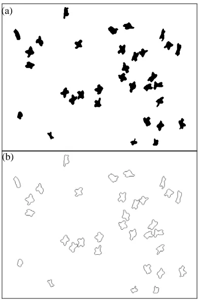
background when it is filled up with black pixels, leaving isolated fiber bodies in white pixels. The flooding also takes away incomplete fibers. Figure 8(a) shows an inversed image of the segmented image, in which the background is in white and fibers in black. Small inner holes or scratches contained in the fiber bodies are removed by using the morphorlogical closing and filling operations [3, 8]. Figure 8(b) displays the fiber boundaries from which cross-sectional areas, perimeters, and shape factors can be calculated [3]. Figure 9 presents a flowchart of major image-processing steps for locating fiber boundaries.
FIGURE 8. Detected fibers (a) and boundaries (b) after removing fiber borders.
FIGURE 9. Flowchart of fiber image processing.
Fifteen images of different fibers were also used to test the fiber detection accuracy of the Otsu algorithm and the dual-thresholding algorithm. The comparison of the two algorithms was listed in Table III. There were a total of 360 valid fibers in the images. The dual-thresholding algorithm was able to correctly detect 88.88% of the fibers, as opposed to 52.78% of Otsu’s accuracy in this case.
TABLE III. Accuracy of fiber detection.
No. of fibers Detected fibers Accuracy
1-D Entropy 360 47 13.1%
2-D Entropy 360 217 60.3%
Minimum
Error 360 57 15.8%
Otsu 360 190 52.78%
Dual-thresholding 360 320 88.88%
CONCLUSION
This paper presents a new fiber segmentation algorithm by using dual thresholds to control image noise and to detect fiber borders that define and separate cross sections for accurate size and shape measurements. The low threshold is selected based on the histogram of the difference from the average grayscale (D) of pixels in the image, and is used to detect only pixels whose D values correspond to the highest frequency in the histogram, avoiding the detection of isolate noise pixels. The pixels detected with the low threshold are the main parts of fiber borders and will be used as seeds in the high-thresholding. The high threshold is computed by a bisection algorithm in conjunction with the low threshold. By recursively tracing the seed pixels in 33 neighborhoods, the expansion of connected pixels lead to complete fiber borders, which are critical for locating accurate fiber cross sections. The experimental results show that the dual-thresholding algorithm can obtain cleaner and more fiber borders than other connectional thresholding algorithms, and improves the detection accuracy from 52.78% and 88.88%.
REFERENCES
[1] Barker, R.L. and Lyons, D.W., Determination of Fiber Cross-Sectional Circularity from Measurements Made in a Longitudinal View. Journal of Engineering for Industry, 101, 59-64, 1979.
[2] Thibodeaux, D.P. and Evans, J. P., Cotton Fiber Maturity by Image Analysis, Textile Research Journal, 56, 130-139, 1986.
[3] Xu, B., Pourdeyhimi, B. and Sobus, J. Fiber Cross-Sectional Shape Analysis Using Imaging Techniques, Textile Research Journal, 63(12), 717-730, 1993.
[4] Matic-Leigh, R. and Cauthen, D. A., Determining Cotton Fiber Maturity by Image Analysis, Part I: Direct Measurement of Cotton Fiber Characteristics, Textile Research Journal, 64, 534-544, 1994.
(a)
(b)
Fiber image
Dual threshold
Boundary extraction Flooding
background
[5] Thibodeaux, D.P. and Rajasekaran, K., Development of New Reference Standards for Cotton Fiber Maturity, Journal of Cotton Science, 3, 188-193, 1999.
[6] Xu, B., Wang, S. and Su, J., Fiber Image Analysis, Part III: Autonomous Separation of Fiber Cross Sections, Journal of Textile Institute, 90, 288-297, 1999.
[7] Hequet, E. and Wyatt, B., Relationship Among Image Analysis on Cotton Fiber Cross Sections, AFIS Measurements and Yarn Quality, the Proceedings of the Beltwide Cotton Conference, 2, 1294-1298, 2001. [8] Xu, B. and Huang, Y., Image Analysis for
Cotton Fibers, Part II: Cross-sectional Measurements, Textile Research Journal, 74(5), 409-416, 2004.
[9] Wan, Y., Yao, L., Xu, B., Wu, X., Separation of Clustered Fibers in Cross-sectional Images using Image Set Theory, Textile Research Journal, 79(18), 1658-1663, 2009.
[10] Wan, Y., Yao, L., Xu, B. and Zeng, P., Shaped Fiber Identification Using A Distance-Based Skeletonization Algorithm, Textile Research Journal, 80(10), 958-968, 2010.
[11] Boylston, E.K., Evans, J.P. and Thibodeaux, D.P., A Quick Embedding Method for Light Microscopy and Image Analysis of Cotton Fibers. J. of Biotechnic and Histochemistry, 70(1), 24-27, 1995.
[12] Boylston, E.K., Thibodeaux, D. P. and Evans, J.P., Applying Microscopy to the Development of a Reference Method for Cotton Fiber Maturity, Textile Research Journal, 63, 80-87, 1993.
[13] Trier, O. D., and Jain, A. K., “Goal-directed evaluation of binarization methods”, IEEE Transactions on Pattern Analysis and Machine Intelligence, 17, 1191-1201, 1995. [14] Ng, Hui-Fuang, “Automatic thresholding for
defect detection”, Pattern Recognition Letters, 27, 1644-1649, 2006.
[15] Kittler, J. and Illingworth, J., On Threshold Selection Using Clustering Criteria, IEEE Transaction on Systems Man Cybernet, 15(55), 652-655, 1985.
[16] Otsu, N., “A threshold selection method from gray-level histogram”, IEEE Transactions on Systems, Man and Cybernetics, 9, 62-66, 1979.
[17] Kapur, J. N., Sahoo, P. K. and Wong, A. K. C., “A new method for gray-level picture thresholding using the entropy of the histogram”, Computer Vision, Graphics and Image Processing, 29(2), 273-285, 1985.
[18] Abutableb, A. S., “Automatic thresholding of gray-level pictures using two-dimensional entropy”, Computer Vision, Graphics, and Image Processing, 47(1), 22-32, 1989.
[19] Kittler, J. and Illingworth J., “Minimum error thresholding”, Pattern Recognition, 19(1), 41-47, 1986.
AUTHORS’ ADDRESSES Yan Wan
Li Yao
Donghua University School of Computer Science Shanghai, Shanghai 200051 CHINA
Bugao Xu