https://doi.org/10.1186/s41546-019-0042-6
R E S E A R C H Open Access
Nonlinear regression without i.i.d. assumption
Qing Xu· Xiaohua (Michael) Xuan
Received: 30 July 2018 / Accepted: 23 September 2019 /
© The Author(s). 2019Open AccessThis article is distributed under the terms of the Creative Commons Attribution 4.0 International License (http://creativecommons.org/licenses/by/4.0/), which permits unrestricted use, distribution, and reproduction in any medium, provided you give appropriate credit to the original author(s) and the source, provide a link to the Creative Commons license, and indicate if changes were made.
Abstract In this paper, we consider a class of nonlinear regression problems without the assumption of being independent and identically distributed. We propose a corre-spondent mini-max problem for nonlinear regression and give a numerical algorithm. Such an algorithm can be applied in regression and machine learning problems, and yields better results than traditional least squares and machine learning methods.
Keywords Nonlinear regression·Minimax·Independent·Identically distributed· Least squares·Machine learning·Quadratic programming
Abbreviations
i.i.d.: Independent and identically distributed MAE: Mean absolute error
MSE: Mean squared error
1 Introduction
In statistics, linear regression is a linear approach for modelling the relationship between a response variableyand one or more explanatory variables denoted byx:
y=wTx+b+ε. (1)
Here,εis a random noise. The associated noise terms{εi}mi=1are assumed to be i.i.d. (independent and identically distributed) with mean 0 and varianceσ2. The parametersw, bare estimated via the method of least squares as follows.
Lemma 1Suppose{(xi, yi)}mi=1are drawn from the linear model (1). Then the
result of least squares is
(w1, w2,· · ·, wd, b)T =A+c.
Here,
A=
⎛ ⎜ ⎜ ⎝
x11 x12 · · · x1d 1
x21 x22 · · · x2d 1 · · · ·
xm1 xm2 · · · xmd 1 ⎞ ⎟ ⎟
⎠, c=
⎛ ⎜ ⎜ ⎝
y1
y2
· · ·
ym ⎞ ⎟ ⎟ ⎠.
A+is the Moore−Penrose inverse1of A.
In the above lemma, ε1, ε2,· · ·, εm are assumed to be i.i.d. Therefore,
y1, y2,· · ·, ymare also i.i.d.
When the i.i.d. assumption is not satisfied, the usual method of least squares does not work well. This is illustrated by the following example.
Example 1Denote by Nμ, σ2 the normal distribution with mean μ and varianceσ2and denote byδcthe Dirac distribution, i.e.,
δc(A)=
1 c∈A,
0 c /∈A.
Suppose the sample data are generated by
yi=1.75∗xi+1.25+εi, i=1,2,· · ·,1517,
where
ε1,· · ·, ε500∼δ0.0325, ε501,· · ·, ε1000∼δ0.5525,
ε1001,· · ·, ε1500∼δ−0.27, ε1501,· · ·, ε1517∼N(0,0.2).
The result of the usual least squares is
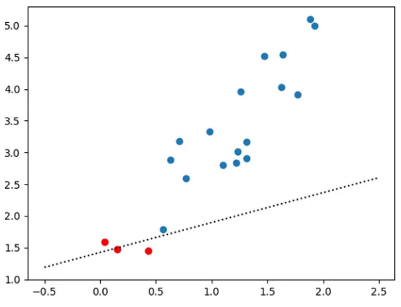
y=0.4711∗x+1.4258,
which is displayed in Fig.1.
We see from Fig.1that most of the sample data deviates from the regression line. The main reason is that the i.i.d. condition is violated.
For overcoming the above difficulty, Lin et al. (2016) studied the linear regression without i.i.d. condition by using the nonlinear expectation framework laid out by Peng (2005). They split the training set into several groups and in each group the i.i.d. condition can be satisfied. The average loss is used for each group and the maximum of average loss among groups is used as the final loss function. They show that the
Fig. 1 Result of least squares
linear regression problem under the nonlinear expectation framework is reduced to the following mini-max problem.
min w,b1≤maxj≤N
1
M
M
l=1
wTxj l+b−yj l 2
. (2)
They suggest a genetic algorithm to solve this problem. However, such a genetic algorithm does not work well generally.
Motivated by the work of Lin et al. (2016) and Peng (2005), we consider nonlin-ear regression problems without the assumption of i.i.d. in this paper. We propose a correspondent mini-max problems and give a numerical algorithm for solving this problem. Meanwhile, problem (2) in Lin’s paper can also be well solved by such an algorithm. We also have done some experiments in least squares and machine learning problems.
2 Nonlinear regression without i.i.d. assumption
Nonlinear regression is a form of regression analysis in which observational data are modeled by a nonlinear function which depends on one or more explanatory variables (see, e.g., Seber and Wild (1989)).
Suppose the sample data (training set) is
S= {(x1, y1), (x2, y2),· · ·, (xm, ym)},
from the hypothesis space{gλ :X →Y|λ∈}such thatgθ(xi)is as close toyias possible.
The closeness is usually characterized by a loss function ϕ such that
ϕgθ(x1), y1,· · ·, gθ(xm), ym attains its minimum if and only if
gθ(xi)−yi=0, 1≤i≤m.
Then the nonlinear regression problem (learning problem) is reduced to an optimization problem of minimizingϕ.
Following are two kinds of loss functions, namely, the average loss and the maximal loss.
ϕ2=
1
m
m
j=1
gθ(xj)−yj
2
.
ϕ∞= max
1≤j≤m
gθ(xj)−yj
2
.
The average loss is popular, particularly in machine learning, since it can be con-veniently minimized using online algorithms, which process fewer instances during each iteration. The idea behinds the average loss is to learn a function that per-forms equally well for each training point. However, when the i.i.d. assumption is not satisfied, the average loss function method may become a problem.
To overcome this difficulty, we use the max-mean as the loss function. First, we split the training set into several groups and in each group the i.i.d. condition can be satisfied. Then, the average loss is used for each group and the maximum of average loss among groups is used as the final loss function. We propose the following mini-max problem for nonlinear regression problems.
min θ 1≤maxj≤N
1
nj nj
l=1
gθ(xj l)−yj l
2
. (3)
Here,nj is the number of samples in groupj.
Problem (3) is a generalization of problem (2). Next, we will give a numerical algorithm which solves problem (3).
Remark 1Jin and Peng (2016) put forward a max-mean method to give the parameter estimation when the usual i.i.d. condition is not satisfied. They show that if Z1, Z2,· · ·, Zkare drawn from the maximal distributionM[μ,μ]and are nonlinearly
independent, then the optimal unbiased estimation forμis
max{Z1, Z2,· · ·, Zk}.
3 Algorithm
Problem (3) is a mini-max problem. The mini-max problems arise in different kinds of mathematical fields, such as game theory and the worst-case optimization. The general mini-max problem is described as
min
u∈Rnmaxv∈V h(u, v). (4)
Here,his continuous onRn×V and differentiable with respect tou.
Problem (4) was considered theoretically by Klessig and Polak (1973) in 1973 and Panin (1981) in 1981. Later in 1987, Kiwiel (1987) gave a concrete algorithm for problem (4). Kiwiel’s algorithm dealt with the general case in whichVis a compact subset ofRd and the convergence could be slow when the number of parameters is large.
In our case,V = {1,2,· · ·, N}is a finite set and we give a simplified and faster algorithm.
Denote
fj(u)=h(u, j )= 1
nj nj
l=1
gu(xj l)−yj l
2
, (u)= max
1≤j≤Nfj(u).
Suppose eachfj is differentiable. Now, we outline the iterative algorithm for the following discrete mini-max problem
min
u∈Rn1≤maxj≤Nfj(u).
The main difficulty is to find the descent direction at each iteration pointuk(k= 0,1,· · ·)since is nonsmooth in general. In light of this, we linearizefjatuk and obtain the convex approximation of as
ˆ
(u)= max
1≤j≤N{fj(uk)+ ∇fj(uk), u−uk}.
Next, we finduk+1, which minimizes (u)ˆ . In general, ˆ is not strictly convex
with respect tou, and thus it may not admit a minimum. Motivated by the alternating direction method of multipliers (ADMM, see, e.g., Boyd et al. (2010) and Kellogg (1969)), we add a regularization term and the minimization problem becomes
min u∈Rn
ˆ
(u)+1
2u−uk
2
.
By settingd=u−uk, the above is converted to the following form
min d∈Rn
max
1≤j≤N{fj(uk)+ ∇fj(uk), d} + 1 2d
2
, (5)
min d,a
1 2d
2+
a
(6)
s.t.fj(uk)+ ∇fj(uk), d ≤a, ∀1≤j ≤N. (7)
Problem (6)−(7) is a semi-definite QP (quadratic programming) problem. When
n is large, the popular QP algorithms (such as the active-set method) are time-consuming. So we turn to the dual problem.
Theorem 1DenoteG= ∇f ∈RN×n, f =(f1,· · ·, fN)T. Ifλis the solution of
the following QP problem
min λ
1 2λ
TGGTλ−fTλ
(8)
s.t.
N
i=1
λi=1, λi≥0. (9)
Thend= −GTλis the solution of problem(6)−(7).
ProofSeeAppendix.
Remark 2Problem(8)−(9)can be solved by many standard methods, such as active-set method (see, e.g., (Nocedal and Wright 2006)). The dimension of the dual problem(8)−(9)is N (number of groups), which is independent of n (number of parameters). Hence, the algorithm is fast and stable, especially in deep neural networks.
Setdk = −GTλ. The next theorem shows thatdkis a descent direction.
Theorem 2Ifdk=0, then there existst0>0such that
(uk+tdk) < (uk), ∀t∈(0, t0).
ProofSeeAppendix.
For a functionF, the directional derivative ofFatxin a directiondis defined as
F(x;d):= lim t→0+
F (x+td)−F (x)
t .
F(x;d)≥0, ∀d∈Rn.
xis called a stationary point ofF.
Theorem2shows that whendk =0, we can always find a descent direction. The next theorem reveals that whendk =0,ukis a stationary point.
Theorem 3Ifdk=0, thenukis a stationary point of , i.e.,
(u
k;d)≥0, ∀d∈Rn.
ProofSeeAppendix.
Remark 3When eachfjis a convex function, is also a convex function. Then,
the stationary point of becomes the global minimum point.
Withdkbeing the descent direction, we use line search to find the appropriate step size and update the iteration point.
Now, let us conclude the above discussion by giving the concrete steps of the algorithm for the following mini-max problem.
min
u∈Rn1≤maxj≤Nfj(u). (10)
Algorithm.
Step 1. Initialization
Select arbitraryu0∈Rn. Setk=0, termination accuracyξ =10−8, gap tolerance
δ=10−7, and step size factorσ =0.5. Step 2. Finding Descent Direction
Assume that we have chosenuk. Compute the Jacobian matrix
G= ∇f (uk)∈RN×n,
where
f (u)=(f1(u),· · ·, fN(u))T.
Solve the following quadratic programming problem with gap toleranceδ (see, e.g., Nocedal and Wright (2006)).
min λ
1 2λ
T
GGTλ−fTλ
s.t.
N
i=1
λi=1, λi≥0.
Step 3. Line Search
Find the smallest natural numberjsuch that
uk+σjdk
< (uk).
Takeαk =σj and setuk+1=uk+αkdk, k=k+1. Go to Step 2.
4 Experiments
4.1 The linear regression case
Example1can be numerically well solved by the above algorithm with
fj(w, b)=(wxj +b−yj)2, j =1,2,· · ·,1517.
The corresponding optimization problem is
min
w,b 1≤maxj≤1517(wxj+b−yj) 2
.
The numerical result using the algorithm in Section3is
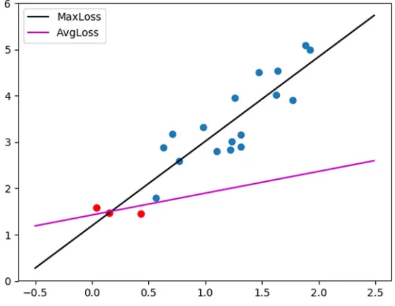
y=1.7589∗x+1.2591.
The result is summarized in Fig.2. Note that the mini-max method (black line) performs better than the traditional least squares method (pink line).
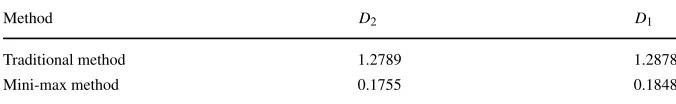
Table 1 Comparisons of the two methods
Method D2 D1
Traditional method 1.2789 1.2878
Mini-max method 0.1755 0.1848
Next, we compare the two methods. Bothl2distance andl1distance are used as measurements.
D2:=
(w− ˆw)2+(b− ˆb)2.
D1:= |w− ˆw| + |b− ˆb|.
We see from table1that mini-max method outperforms the traditional method in bothl2andl1distances.
Lin et al. (2016) have mentioned that the above problem can be solved by genetic algorithms. However, the genetic algorithm is heuristic and unstable especially when the number of groups is large. In contrast, our algorithm is fast and stable and the convergence is proved.
4.2 The machine learning case
We further test the proposed method by using the CelebFaces Attributes Dataset (CelebA)2 and implement the mini-max algorithm with a deep learning approach. The dataset CelebA has 202599 face images among which 13193 (6.5%) have eye-glass. The objective is eyeglass detection. We use a single hidden layer neural network to compare the two different methods.
We randomly choose 20000 pictures as the training set among which 5% have eye-glass labels. For the traditional method, the 20000 pictures are used as a whole. For the mini-max method, we separate the 20000 pictures into 20 groups. Only 1 group contains eyeglass pictures while the other 19 groups do not contain eyeglass pictures. In this way, the whole mini-batch is not i.i.d. while each subgroup is expected to be i.i.d.
The traditional method uses the following loss
loss= 1 20000
20
i=1 1000
j=1
(σ (W xij+b)−yij)2.
The mini-max method uses the maximal group loss
loss= max
1≤i≤20
1 1000
1000
j=1
(σ (W xij +b)−yij)2.
Here,σ is an activation function in deep learning such as the sigmoid function
σ (x)= 1
1+e−x.
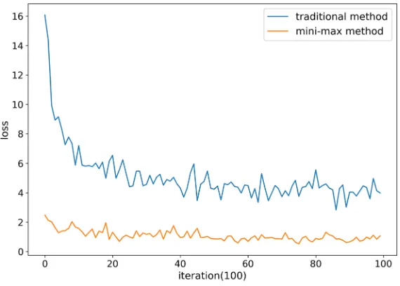
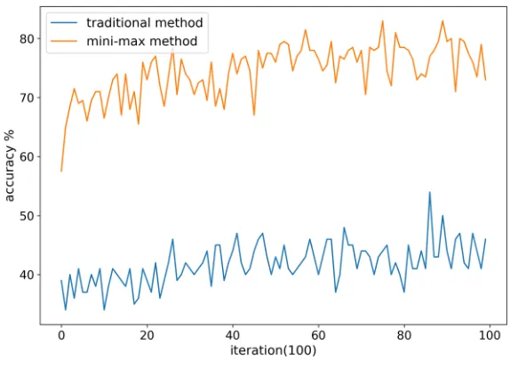
We perform the two methods for 100 iterations. We see from Fig.3that the mini-max method converges much faster than the traditional method. Figure4also shows that the mini-max method performs better than the traditional method in accuracy. (Suppose the total number of the test set isn, andmof them are classified correctly. Then the accuracy is defined to bem/n.)
The average accuracy for the mini-max method is 74.52% while the traditional method is 41.78%. Thus, in the deep learning approach with a single layer, the mini-max method helps to speed up convergence on unbalanced training data and improves accuracy as well. We also expect improvement with the multi-layer deep learning approach.
5 Conclusion
In this paper, we consider a class of nonlinear regression problems without the assumption of being independent and identically distributed. We propose a corre-spondent mini-max problem for nonlinear regression and give a numerical algorithm. Such an algorithm can be applied in regression and machine learning problems, and yields better results than least squares and machine learning methods.
Fig. 4 Accuracy of the two methods
Appendix
Proof of Theorem1
Consider the Lagrange function
L(d, a;λ)=1
2d
2+
a+
N
j=1
λj(fj(uk)+ ∇fj(uk), d −a).
It is easy to verify that problem (6)−(7) is equivalent to the following minimax problem.
min
d,a maxλ≥0L(d, a;λ).
By the strong duality theorem (see, e.g., (Boyd and Vandenberghe2004)),
min
d,a maxλ≥0L(d, a;λ)=maxλ≥0mind,a L(d, a;λ).
Sete=(1,1,· · ·,1)T, the above problem is equivalent to
max λ≥0mind,a
1 2d
2+a+λT(f+Gd−ae)
.
Note that
1 2d
2+a+λT(f +Gd−ae)=1 2d
If 1−λTe= 0, then the above is−∞. Thus, we must have 1−λTe=0 when the maximum is attained. The problem is converted to
max λi≥0,Ni=1λi=1
min d
1 2d
2+λTGd+λTf
.
The inner minimization problem has the solution d = −GTλ and the above problem is reduced to
min λ 1 2λ T
GGTλ−fTλ
s.t.
N
i=1
λi=1, λi≥0.
Proof of Theorem2
Denoteu=uk, d=dk. For 0< t <1,
(u+td)− (u)
= max
1≤j≤N{fj(u+td)− (u)}
= max
1≤j≤N{fj(u)+t∇fj(u), d − (u)+o(t)}
≤ max
1≤j≤N{fj(u)+t∇fj(u), d − (u)} +o(t)
= max
1≤j≤N{t (fj(u)+ ∇fj(u), d − (u))+(1−t)(fj(u)− (u))} +o(t)
Note thatfj(u)≤ (u)= max
1≤k≤Nfk(u)
≤t max
1≤j≤N{fj(u)+ ∇fj(u), d − (u)} +o(t).
Sincedis the solution of problem (5), we have that
max
1≤j≤N
fj(u)+ ∇fj(u), d + 1 2d
2
≤ max
1≤j≤N
fj(u)+ ∇fj(u),0 + 1 20
2
= max
Therefore,
max
1≤j≤N{fj(u)+ ∇fj(u), d − (u)} ≤ − 1 2d
2
.
⇒ (u+td)− (u)≤ −1
2td
2+o(t).
⇒ (u+td)− (u)
t ≤ −
1 2d
2+
o(1).
⇒ lim sup t→0+
(u+td)− (u)
t ≤ −
1 2d
2
<0.
Fort >0 small enough, we have that
(u+td) < (u).
Proof of Theorem3
Denoteu=uk. Then,dk =0 means that∀d,
max
1≤j≤N{fj(u)+ ∇fj(u), d} + 1 2d
2≥
max
1≤j≤Nfj(u). (11) Denote
M= max
1≤j≤Nfj(u). Define
=
j|fj(u)=M, j =1,2,· · ·, N
.
Then (see Demyanov and Malozemov (1977)) (u;d)=max
j∈∇fj(u), d. (12)
Whendis small enough, we have that
max
1≤j≤N{fj(u)+ ∇fj(u), d}
=max
j∈{fj(u)+ ∇fj(u), d}
=M+max
j∈∇fj(u), d.
In view of (11), we have that fordsmall enough,
max
j∈∇fj(u), d + 1 2d
2≥
0.
For anyd1∈Rn, by takingd=rd1with sufficient smallr >0, we have that
max
j∈∇fj(u), rd1 +
r2
2d1
2≥
0.
max
j∈∇fj(u), d1 +
r
2d1
2≥0
Letr→0+,
max
j∈∇fj(u), d1 ≥0. Thus, we fulfill the proof by combining with (12).
Acknowledgements The authors would like to thank Professor Shige Peng for useful discussions. We especially thank Xuli Shen for performing the experiment in the machine learning case.
Authors’ contributions
MX puts forward the main idea and the algorithm. QX proves the convergence of the algorithm and collects the results. Both authors read and approved the final manuscript.
Funding
This paper is partially supported by Smale Institute.
Availability of data and materials
Please contact author for data requests.
Ethics approval and consent to participate
Not applicable.
Consent for publication
Not applicable.
Competing interests
The authors declare that they have no competing interests.
References
Ben-Israel, A. and T.N.E. Greville. (2003).Generalized inverses: Theory and applications (2nd ed.), Springer, New York.
Boyd, S., N. Parikh, E. Chu, B. Peleato, and J. Eckstein. (2010).Distributed Optimization and Statistical Learning via the Alternating Direction Method of Multipliers, Found. Trends Mach. Learn.3, 1–122. Boyd, S. and L. Vandenberghe. (2004).Convex Optimization, Cambridge University Press.https://doi.org/
10.1017/cbo9780511804441.005.
Demyanov, V.F. and V.N. Malozemov. (1977).Introduction to Minimax, Wiley, New York.
Jin, H. and S. Peng. (2016).Optimal Unbiased Estimation for Maximal Distribution.https://arxiv.org/abs/ 1611.07994.
Kellogg, R.B. (1969).Nonlinear alternating direction algorithm, Math. Comp.23, 23–38.
Kendall, M.G. and A. Stuart. (1968).The Advanced Theory of Statistics, Volume 3: Design and Analysis, and Time-Series (2nd ed.), Griffin, London.
Kiwiel, K.C. (1987).A Direct Method of Linearization for Continuous Minimax Problems, J. Optim. Theory Appl.55, 271–287.
Legendre, A.-M. (1805).Nouvelles methodes pour la determination des orbites des cometes, F. Didot, Paris.
Lin, L., Y. Shi, X. Wang, and S. Yang. (2016).k-sample upper expectation linear regression-Modeling, identifiability, estimation and prediction, J. Stat. Plan. Infer.170, 15–26.
Lin, L., P. Dong, Y. Song, and L. Zhu. (2017a).Upper Expectation Parametric Regression, Stat. Sin.27, 1265–1280.
Lin, L., Y.X. Liu, and C. Lin. (2017b).Mini-max-risk and mini-mean-risk inferences for a partially piecewise regression, Statistics51, 745–765.
Nocedal, J. and S.J. Wright. (2006).Numerical Optimization, Second Edition, Springer, New York. Panin, V.M. (1981).Linearization Method for Continuous Min-max Problems, Kibernetika2, 75–78. Peng, S. (2005).Nonlinear expectations and nonlinear Markov chains, Chin. Ann. Math.26B, no. 2,
159–184.