Linear or non Linear modeling for ENSO dynamics?

Linear or NonlinearModeling for ENSO Dynamics?

Marco Bianucci1,*, Antonietta Capotondi2, Riccardo Mannella3and Silvia Merlino1 1 _{ISMAR-CNR, 19032 La Spezia Italy; [email protected]}

2 _{University of Colorado, CIRES, 80309 Boulder (CO) USA, and}

NOAA-ESRL, Physical Sciences Division, 80305 Boulder (CO) USA; [email protected] 3 _{Physics Department, Pisa University, 56127 Pisa Italy; [email protected]}

* Correspondence: [email protected]

Abstract: The observed ENSO statistics exhibits a non-Gaussian behavior, which is indicative of the presence of nonlinear processes. In this paper, we use the Recharge Oscillator Model (ROM), a largely used Low-Order Model (LOM) of ENSO, as well as methodologies borrowed from the field of statistical mechanics to identify which aspects of the system may give rise to nonlinearities that are consistent with the observed ENSO statistics. In particular, we are interested in understanding whether the nonlinearities reside in the system dynamics or in the fast atmospheric forcing. Our results indicate that one important dynamical nonlinearity often introduced in the ROM cannot justify a non-Gaussian system behavior, while the nonlinearity in the atmospheric forcing can instead produce a statistics similar to the observed. The implications of the non-Gaussian character of ENSO statistics for the frequency of extreme El Niño events is then examined.

Keywords: non-Hamiltonian complex systems; Fokker–Planck equation; transport coefficients; El Niño-La Niña; Lie evolution; projection approach

1. Non-Gaussian-Nonlinear Features of the ENSO Statistics

It is well established that some aspects of the El Niño Southern Oscillation (ENSO) have a non-Gaussian statistics, a characteristic that is indicative of some underlying nonlinear process. For example, the plot of the frequency of the Niño 3 index (averaged Sea Surface Temperature (SST) anomalies in the region 5◦S–5◦N, 150◦W–90◦W) shows that the likelihood of large positive SST anomalies is greater than that of negative anomalies (Figure1), indicating that the SST anomalies achieved in the eastern equatorial Pacific during the mature phase of an El Niño are larger than those occurring during la Niña events. Another asymmetry is the duration of the transition from one ENSO phase to the other, with a rapid transition from El Niño to La Niña, but a slower transition from La Niña to El Niño [1]. The duration of El Niño events tends to be shorter than that of La Niña ones, and the range of El Niño flavors is larger than that of La Niña [2].

This non-Gaussian behavior is quantified by the positive skewness of the SST distribution: γ1 ∼0.7. A positive kurtosisγ2∼ 1.1 also clearly indicates that extreme events are more likely to

occur than for a normal distribution.

The non-Gaussianity of the histogram arises from non-linear contributions in the equation of motion governing the system, and it is important to understand which nonlinearities play the most relevant role in the ENSO evolution. We know that ENSO is the result of complex large-scale ocean-atmosphere interactions that also include non-linear processes. For instance, An and Jin [3] proposed that the Nonlinear Dynamical Heating (NDH) in the ocean mixed layer is crucial for generating intense El Niño events, mainly due to the vertical nonlinear advection. Asymmetries in intensity can also result from ocean-atmosphere coupling processes (e.g., [4]) or from the nonlinear response of the zonal wind stress to ENSO SST anomalies [5,6]. In general, the complexity of the ENSO, as for most of the large-scale phenomena resulting from the ocean-atmosphere interaction, makes it challenging to understand the general key features of the statistics and dynamics of the events. Thus, to mimic the highly complex nature of ENSO events, as the diversity in spatial flavors

and the “non-normal” growth of fluctuations [7], large multivariate linear models with multivariate additive stochastic perturbations have been exploited [8,9]. Here, we focus instead on Low Order Models (LOMs), i.e., the set of Ordinary Differential Equations (ODE) for ENSO, perturbed by a fast and chaotic forcing. Probably, a more realistic modeling of ENSO should merge these two pictures (multidimensionality and nonlinearities). A deeper discussion about the effective and respective roles of the dimension and of the nonlinearities of an LOM to model the complexity of ENSO goes beyond the task of the present work.

The tropical Pacific can be well described by shallow water equations driven at the surface by the easterly trade winds, thus allowing for a drastic simplification of the system dynamics.

Simple shallow water equations together with the assumption of a large timescale separation between the ENSO dynamics and the typical dynamics of atmospheric processes make it possible to reduce the description of the dynamics of the ENSO-relevant variables, to a relatively simple LOM. This LOM can be separated in a slow part, or “system of interest”, associated with the slow evolution of oceanic variables like SST and thermocline depth, and a fast “rest of the system” that primarily includes fast atmospheric processes, e.g., the Madden–Julian Oscillation (MJO), the Westerly Wind Bursts (WWBs), etc., which are considered important in forcing ENSO. ENSO LOMs that have been extensively considered in the literature include the Recharge Oscillator Model (ROM, e.g., [10–17] among many others) and the Delayed Oscillator (DO, e.g., [18,19]). In these models, ENSO events are triggered by the forcing provided by the fast atmospheric variables, which are usually represented as a stochastic perturbation of the system of interest.

The simplified representation of ENSO in the LOMs provides a suitable framework for examining the impact of the system nonlinearities on the ENSO statistics. In particular, an important question is whether the relevant nonlinearities reside in the interaction among the variables of the system of interest (dynamical nonlinearities), as suggested, for example in [18], or are associated with the interaction of the system of interest with the atmospheric fast forcing, as indicated, among others, by [6,20].

The fast atmospheric forcing can be included in two ways: considering this forcing as stochastic or assuming a deterministic motion with initial conditions distributed according to some distribution (the Gibbs idea of ensemble). The former approach is often used in the oceanographic field, where the dynamics is divided into a slow and a very fast and chaotic component, and the fast part is considered to be random (usually modeled as white noise) [21–25]. The latter approach has been largely used in the context of the foundation of statistical mechanics and thermodynamics and, more recently, also in the oceanographic field by some of the authors [17,26,27]. It aims at starting from more realistic deterministic systems (instead of the stochastic ones), and by using projection- perturbation procedures, it allows managing also the cases in which the time scale separation between the dynamics of the part of interest and that of the rest of the system is not so large: this is the reason why in this work, we shall focus on the projection-perturbation approach, which has been applied to the multi-scale ENSO system.

Both approaches have their strengths and weaknesses, and a large literature has been devoted to justify both from a formal and theoretical point of view (for a review about the foundation of the stochastic approach, see [28], and for the projection approach, see, e.g., [29–33]). It is far beyond the scope of the present work to discuss the foundation of these approaches. However, both aim at obtaining a Partial Differential Equation (PDE), ideally a Fokker–Planck Equation (FPE), guiding the dynamics of the Probability Density Function (PDF) for the variables of the part of interest of the system.

is possible to obtain statistical information about the quantity of interest. For example, the FPE is the major approach for determining, both analytically and numerically, important quantities like the First Passage Time (FPT; see for example [40]), in a variety of contexts ranging from civil and mechanical engineering, physical chemistry [41–43], disordered systems [44,45], neuroscience [46,47], biochemistry [48], biomedicine, mathematical financing, image processing, computer science, etc.

More generally, the possibility of using an FPE to model the statistical behavior of the relevant properties of the variables of interest is often crucial because the FPE is the only non-trivial partial differential equation that in many cases can be approached for a solution with analytical tools, and it looks like a Schrodinger equation [49]. In the present paper, we shall obtain a general FPE for the perturbed linear/non-linear ROM representing the ENSO dynamics, and we will compare some general statistical features resulting from the FPE (such as the stationary PDF, the relaxation properties and the average timing of the events) with observations, to infer the specific nature of the nonlinearities of the ENSO modeled by the ROM.

p

(T)

0

0.9

1.8

2.7

-2.7

-1.8

-0.9

NINO3 1950-2014

THREE-MONTH AVERAGE

0.5

0.4

0.3

0.2

0.1

Figure 1.Histogram of the frequency for the three-month average Niño 3 data from NOAA [50]. The dashed line is the best fit of the stationary PDF found in [17] (strongly skewed and with a heavy tail), and solid blue line is a normal distribution with the same average and variance of the observation data.

comparing them with the theoretical ones. The aim is to assess where the nonlinearities responsible for the non-Gaussian features of the ENSO statistics reside. Section7is devoted to discussing the results and drawing conclusions.

2. The Dynamics of the Components of the ENSO: The Recharge Oscillator Model

The El Niño Southern Oscillation, also known as ENSO, is a periodic fluctuation of the SST (El Niño) and the sea level pressure (Southern Oscillation) across the equatorial Pacific Ocean. The fluctuations arise over a normal condition of strong SST gradient between the east (cold tongue) and the west (warm pool) equatorial Pacific Ocean. ENSO is a complicated, not yet fully-understood, coupled ocean-atmosphere phenomenon in which basin-wide changes in sea surface temperatures, trade winds and atmospheric convection are intimately related. However, the particular ocean and atmosphere conditions that generate, and in some way also define, the El Niño/La Niña events allow the representation of the key ocean-atmospheric feedbacks responsible for this complex phenomenon in a simplified fashion.

The upper layer of the tropical Pacific Ocean, responsible for the energy and momentum exchange with the atmosphere, is a very long strip of water with a meridional width of a few hundred kilometers, a zonal extension of about 10,000 km and an average depth of about 120 m, as defined by the depth of the thermocline. The water in this strip flows over the deeper and colder ocean, from the South American coasts to the warm Asian coasts, mainly driven by the easterly trade winds and “trapped” in the convergence ocean zone, around the equatorial latitude, ultimately due to the Coriolis effect.

This motion accumulates warm water in the western Pacific Ocean, and because of the closed eastern boundary, it forces the cold and deep water to rise up in the eastern Pacific to compensate the surface water moving westward. This process generates the strong SST gradient between the two sides of the basin, which, in normal conditions, is in equilibrium with the easterly trade winds.

During an El Niño (La Niña) event, this SST gradient from east to west is reduced (increased): we consider that an El Niño (La Niña) event is occurring when the SST anomaly on the east equatorial Pacific is greater (lesser) than 0.5 (−0.5) degrees Celsius with respect to the average value. The SST anomalies are related to the thermocline depth anomalies. Thus, the key quantities that characterize ENSO in the equatorial Pacific Ocean are the SST anomaly (TE) in the eastern part of the domain,

usually described in terms of the Niño 3index (average SST in the area 5◦ S–5◦N, 150◦W–90◦W), and the zonal average of the anomaly of the thermocline depth (h).

Exploiting these very peculiar physical conditions of the equatorial surface layer of the Pacific Ocean and from two-box (east and west side, respectively), two-strip (equatorial and off equatorial, respectively) approximations of the shallow water Navier–Stokes (NS) equations applied to the tropical Pacific Ocean, Jin obtained the following very simple system of linear equations for the Pacific equatorial thermocline depth anomaly [10,11]:

˙

hW=−r hW−α τs (1a)

hE−hW=τs (1b)

whereτs is the zonally-integrated wind stress anomaly, the subscriptW(E) means that the variables

refer to the west (east) side of the basin, the friction termrcollectively represents the damping of the upper ocean system through mixing and the equatorial energy loss to the boundary layer currents at the east and west sides of the ocean basin, and it is set in the range 6.3 month.r−1_{.8.0 months [10,11].}

linear system is about zero at the equilibrium state, that is,hE+hW =0 (at equilibrium), then from

Equation (1), one finds thatαshall be about half ofr.

The work in [10,11] provided a physical basis for the simple linear relationships in Equation (1), in the long wave, two-strip approximation.

Notice that if the wind stressτswere a fast forcing completely independent of the dynamics of

the thermocline depth anomaly, Equation (1) would give rise to a very simple relaxation process with relaxation time given by 1/r, which, of course, is not what happens in reality. In fact, as we shall see below, the wind dynamics has a slow part that is strongly correlated with the dynamics ofhvia a direct linear relationship with the other ENSO variable: the SST anomalyTE.

A linear ODE for the thermodynamics relationship between the variation of the anomalous SST and the thermocline depth was proposed in [10,11,52,53] and related subsequent works:

˙

TE=−c TE+γhE+δSτs,E. (2)

where the first term on the right-hand side is a damping process with a collective damping ratec. The second term describes the influence onTEof the thermocline displacement, andδSis the Ekman

pumping coefficient of the vertical advective feedback processes due to the wind stress averaged over the domain, which actually can be considered vanishing (see [10,52,53] for details):δS =0.

Using Equation (1b), we can rewrite Equation (2) as: ˙

TE=−c TE+γhW+γ τs. (3)

The above equation relates the dynamics ofTE to that of hW. However, as we have already

observed, also the dynamics ofhW, given in Equation (1), depends on the values of theTEvariable.

This dependence is due to the fact that the wind stressτs is strongly influenced by the zonal SST

gradient. In effect, in most of the works on the ROM [52,53] and on the DO [18], it is explicitly assumed that the following linear relationship holds true:

τs=b TE+g(t), (4)

where g(t)is a fast “chaotic” fluctuating function of time. In this work, we define as “chaotic” a unidimensional function of timeg(t)if its dynamics can be considered “almost ” random so as to allow us to substitute it safely with a genuine stochastic process or to use a second-order perturbation projection approach, as hereafter specified. In the first case, we should exploit well-known works about limit theorems (e.g., [54]) and introduce a more specific chaotic hypothesis (e.g., [55,56]) that, actually, has been proven to be satisfied only by highly idealized mathematical models. In the second case, the requests are less stringent, because it is enough that for anyn∈_N, the correlation function hg(t)g(t+t1)...g(t+tn)idecays “quickly enough” for each 1 ≤k≤ n, to avoid divergences in the

neglected terms obtained with the perturbation procedure [29,57–59]. The extensive use of the quotes is to stress the fact that, as already stated in the Introduction, it is beyond the focus of the present work to discuss the dynamical foundation of stochastic processes/statistical mechanics. For further use, we specify that the symbolh...iindicates a time average:hai:=limT→∞R0Ta(t)dt/T, but we shall exploit

the ergodic assumption and the Gibbs idea to turn the time averages into ensemble averages. Equation (4) implies that the slow component of the wind stress and the slow component ofTE

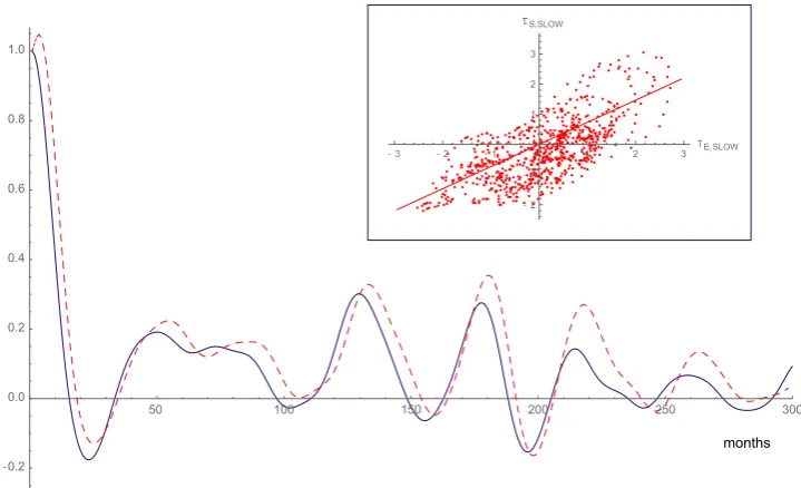
are proportional to each other. Figure 1 of the paper [60] supports this assumption, and we further validate this hypothesis by analyzing the NOAA data [61], as detailed in AppendixA, where the wind stress anomalyτsis divided into slow (τ_s,slow) and fast (τ_{s,f ast}) components. Theτ_s,slowdata are obtained from the one-year average ofτsdata, whileτs,f ast ≡τs−τs,slowcan be identified withg(t)

of (4).

˙

hW=−rhW−αbTE−αg(t)

˙

TE=γhW−λTE+γg(t), (5)

withλ≡c−γb.

Considering thatαis quite smaller thanγ[10,11], we disregard the forcing term−αg(t)in the first equation of System (5), and finally, we are led to the following simplified linear ROM:

˙

hW =−rhW−αbTE

˙

TE=γhW−λTE+g(t) (6)

where we have included the constantγin the definition of the fast partg(t)of the wind stressτs.

The result of Equation (6) is really remarkable because it is a very simple, but still informative, description of a complex large-scale ocean/atmosphere process. We can consider it on the same footing as the Onsager linear regression principle, chemical reaction rate models [43] and other linear results of standard thermodynamics and statistical mechanics, which arise as large time and space scale phenomena from an underlying complex fast and chaotic dynamics.

3. Is a Possible Internal Nonlinearity Relevant?

Because of the linear relationship betweenhEandTEof Equation (2), the “internal” dynamics (i.e.,

forg(t) =0) of the ROM of Equation (6) is, by construction, linear. However, a linear relationship in the real world is almost always an approximation; thus in this section, we analyze the possibility that a nonlinear correction is effectively present in the interaction between the thermocline depth anomaly and the SST anomaly, and we try to evaluate if this correction can contribute to the non-Gaussian features of the ENSO. Actually, in [18], it is argued that a nonlinear cubic relationship between the anomalous subsurface temperatureTsuband the thermocline depth anomaly should be taken into

account:

Tsub=a hE−e∗h3E+O(h5E), (7)

where the values for the coefficientsaande∗have been roughly estimated in [18] asa∼0.14◦C m−1 ande∗ ∼3×10−5◦_{C m}−3_{. From this nonlinear relation, a small cubic term inh}

Ewould enter also in

Equation (2) [18]. Given the very small value of the ratioe∗/a, the cubic term should play some role only forhE≥ ±2σ_hE(σ_hEis the standard deviation ofhEthat is a little over 10 m [62]), reaching the same

value of the linear term for abouthE ∼

√

a/e∗_{=36 m (about 3σ}

hE). Using these arguments, in [63], it has been already shown that assuming a nonlinear ROM linearly interacting with the atmosphere, we obtain a non-normal stationary PDF. However, as we can see in Figure. 5 of [60], both observations and numerical results show that the relationship betweenTsub andh is far more linear than what

was suggested in [18]. In fact, this figure shows a small dispersion of the data around the linear fit, for a range of values ofhEthat spans beyond±4σhE. Thus, we have evidence, from observations, that the nonlinear correction to the linear ROM is quite smaller that the (already small) value estimated in [18]. However, to evaluate the relevance of this small nonlinear term for the ENSO statistics, we also have to account for the behavior of the PDF for large values ofh. To estimate the PDF including the nonlinear correction in the interaction between the thermocline depth anomaly and the SST anomaly, we consider the following nonlinear ROM:

˙

hW=−rhW−αbTE

˙

TE=γU0(hW)−λTE+g(t), (8)

in which

where for a generic function f(x), we have defined f0(x) := d f(x)/dxandκ is a parameter that, according to the above results, is much smaller than the value of the ratioe∗/a, i.e.,κ<<10−4m−2. The stationary PDF that can be derived from Equation (8), consideringg(t)as an additive fast fluctuating forcing, is as follows. We change variables:v≡ −rhW−αbTE,x=hW, and Equation (8) becomes:

˙ x=v

˙

v=−αbγU0(x)−λr x−(r+λ)v−αb g(t). (10) Ifg(t)is assumed to be a white noise with a correlation functionhg(0)g(t)i=2dδ(t), Equation (10) describes the dynamics of a particle with coordinatex, velocityv, in an “almost” harmonic potential given by:

V(x) =αbγU(x) +λrx

2

2 '(λr+αbγ) x2

2 +αbγ κ x4

4 (11)

and interacting with a thermal bath with frictionr+λand “temperature”Θ=α2b2d/(r+λ). It is well known that the stationary PDF for such a system is the “canonical” one:

ρs(x,v) =Z e−

H(x,v)

Θ _{, (12)}

whereZis the normalization constant andH(x,v) ≡V(x) +v₂2 is the Hamiltonian. Thus,Θis the variance of the “velocity” variablev: Θ=hv2is ≡σ_v2. As for thex(= hW) variable, we notice that,

given the small value of theκparameter, the non-harmonic termαbγ κx4/4 in the potentialV(x)of Equation (11) gives a negligible contribution to the variance; thus, we also haveΘ'(λr+αbγ)hx2is :=

(λr+αbγ)σ_x2. Therefore, the stationary PDF of Equation (12) is very well approximated by a Gaussian function until the nonlinear term of the potentialαbγ κx₄4 enters into play, but, as already noted, this happens whenx = hW far exceeds at least two standard deviations, i.e., where the non-Gaussian

feature could not really emerge because of the extremely low value of the PDF of Equation (12). Thus, we are led to the conclusion that the possibly nonlinear interaction between the internal ROM variables cannot inherently be the cause of the observed non-Gaussian properties of the ENSO statistics.

Notice that if we consider the external forcingg(t)as a correlated noise (i.e., not white) or as a weak deterministic chaotic perturbation with a finite time scale (namely, with correlation function that decays in a finite time), using a Zwanzig-like projection approach in the perturbation version of [64–66], we obtain a stationary PDF for the ROM variables that is similar to the one in Equation (12), apart from some small changes in the parameterΘand in the coefficients of the potentialV(x). Thus, also in these non-Markovian cases, the same argument of the previous white noise case applies: the non-Gaussian features of the PDF would be negligible and not as pronounced as observed.

So far, we have shown that analyzing the relations between the dynamics ofhWandTE, it is hard

to find nonlinearities strong enough to justify the non-Gaussian behavior of the ENSO statistics. Thus, from now on, we shall assume that the non-harmonic term in the potentialU(hW)of Equation (9)

can be neglected. Namely, we return to the linear ROM of Equation (6) and attempt to justify the observed nonlinearities focusing on the interaction of the slow components of the ROM of Equation (6) withg(t).

It is worthwhile to remark that a recent study [67] has highlighted the importance of the nonlinear advective terms in the upper-ocean temperature equations as a source of ENSO nonlinearities and the resulting non-Gaussianity of eastern Pacific SST anomalies. These nonlinear advective terms, which have been collectively termed Nonlinear Dynamical Heating (NDH), are primarily controlled by the anomalies of the zonal advection term (u0∂xT0; see [67] for the nomenclature). However,

Before doing that, however, we simplify Equation (6) a little in the following way: ˙

h=−ωTE

˙

TE=ωh−λTE+g(t), (13)

whereh≡(hW+hE)/2 is the zonally-averaged thermocline depth anomaly (directly related to the

anomalous heat accumulated in the Equatorial Pacific Ocean), a choice justified by the arguments and results of [12], shortly summarized hereafter. First, Equation (1b) implies that the tilt of the thermocline reacts almost instantaneously to wind stress, but it is more realistic to assume that the adjustment of the thermocline depth takes a finite time, approximately the time it takes for a Kelvin wave to propagate from the western central Pacific to the east. Thus, Equation (1b) should be replaced by:

˙

hE=−γh(hE−hW−τs).

Second, repeating the same steps that led us from Equation (1b) to Equation (6), we get an unperturbed ROM given by three differential equations that better represent the ENSO dynamics, leading to a better agreement among the parameter of the model and observations. Finally, studying in detail the feature of this linear three-degrees of freedom system, we see that one eigenstate has a fast decay time (shorter than one month); thus, the dynamics is attracted toward a two-dimensional slow manifold, well represented by the reduced ROM of Equation (13).

Suitable values forωandλ(the “friction” coefficient) can be obtained by using phenomenological considerations when deriving the ROM from building block equations and/or directly from a fit to observations (see [12]). In the literature, we find different values that range from 2π/48 month−1–2π /36 month−1forωand from 1/12 month−1–1/6 month−1forλ. We shall see in the following that we

can shrink these ranges.

4. The Multiplicative Nature of the Forcing

In some recent works, it has been shown that to account for the instability of the dynamics, the skewness and the tail of the observed stationary PDF of the ENSO, the perturbation forcingg(t)of the ROM cannot be simply additive, but a multiplicative term, directly correlated with the additive one, should also be considered [14,15,17], leading to a perturbation of the form:

g(t) =e(1+βTE)ξ(t), (14) whereξ(t)is a fast chaotic fluctuating term andeis a parameter that controls the strength of the interaction. Many facts support the hypothesis given by Equation (14):

• the multiplicative nature of the ENSO forcing provided by the Madden–Julian Oscillation (MJO) and its higher frequency tail ([68,69] and the references therein);

• multiplicative fast forcings typically emerge from the general perturbation approaches to large-scale ocean dynamics [70,71];

• considering the nonlinear nature of the heat budget equation for the surface mixed layer [72], we get multiplicative fast fluctuations in both the net surface/subsurface heat flux and the advective contributions [16,67,70,71].

Concerning the last point, we again notice that the equatorial Pacific zonal subsurface NDH u0∂xT0, which plays a role in the asymmetry of the El Niño-La Niña events [67], may be linked to the

multiplicative termeβTEξ(t)of Equation (14), assuming thatξ(t)andTEare directly related tou0and

∂xT0, respectively.

Thus, inserting Equation (14) into the ROM of Equation (13), we get: ˙

h=−ωTE

˙

that is the final model we shall take into account hereafter.

When ξ(t) is a white noise, the term (1 + βTE)ξ(t) is often named Correlated-Additive-Multiplicative (CAM) noise [21–23], but we shall extend this notation also to deterministic (i.e., not stochastic) processes, saying that(1+βTE)ξ(t)is a CAM forcing. In Section6, starting from observations, we shall use a statistical inference method for diffusion processes with nonlinear drift to estimate the effective contribution of the CAM forcing with respect to a more simple additive fast forcing.

In general, it is reasonable that at least a part of the additive forcing should not be correlated with the multiplicative one, i.e., that there are different independent fast chaotic forcings that can be collected as an independent additive contribution, uncorrelated to the previous one, considered above: g(t) = f(t) + (1+βTE)ξ(t), (16) where f(t)is uncorrelated withξ(t). However, for the sake of simplicity, we do not consider this possibility here. This more general ROM will be examined in a subsequent paper.

We want to stress again that we do not make the assumption that the forcing term ξ(t) of Equation (15) has a stochastic nature. ξ(t) is a deterministic “chaotic” forcing, and statistics is introduced by using the Gibbs concept of ensemble (our PDF).

5. The Fokker–Planck Equation Guiding the Statistics of the ROM

The ROM of Equation (15) must be validated by observations of the ENSO, namely we must use some data analysis approach to infer the values of the coefficients of the ROM of Equation (15). Due to the multiplicative character of the perturbation, the system is not linear; thus, strictly speaking, well consolidated approaches based on the Gaussian properties of the data dispersion, such as the Linear Inversion Model (LIM), cannot be used in this case. However, as will be shown in the next section, if we observe only, or if we are interested only in the first (the mean) and the second (the variance) moments, then the system of Equation (15) looks to be linear, with eigenvalues that are weakly renormalized by theβparameter. Of course, replacing the nonlinear ROM of Equation (15) with a linear one, all the information concerning large deviations from the averages will be lost. Because we are interested in evaluating the role of the nonlinearities in the ENSO dynamics, modeled by the perturbed ROM, we would need an FPE for the PDF of the SST anomalies that fully retains the nonlinear nature of the interaction between the ENSO variables of interest(h,TE)and the collective variable

ξ(t)of Equation (15). In this way, in fact, a comparison between the FPE predictions and observations should possibly validate the model and allow one to estimate the relative weight of the multiplicative perturbation. In this section, we briefly recall and use some of the results of [17,26,27,32,33] to introduce an explicit FPE for the PDF of the ROM system.

∂tσ(h,T;t) =ω ∂hT−ω ∂Th+λ ∂TT+Dβ ∂T(1+βT) +∂TD(1+βT)2∂T σ(h,T;t)

=

ω ∂hT−ω ∂Th+λ ∂TT−Dβ ∂T(1+βT)

+∂2_TD(1+βT)2 σ(h,T;t) (17) whereD≡e2hξ2iτis the “standard” diffusion coefficient.

In the case where the time scale separation between the unperturbed ROM and the fast forcing is not so extreme, as we have already stressed, we cannot approximate the deterministic forcingξ(t) with a white noise, and we have to work with ensembles (i.e., PDF) for which the time evolution is guided by the Liouvillian corresponding to the equation of motion of the perturbed ROM of Equation (15). Starting from the Liouville equation, assuming weak perturbation of the ROM (small evalues) and using a projection perturbation approach, it is thus possible to derive an effective FPE that well approximates the dynamics of the PDF [17] (see also AppendixBfor a short summary of the projection procedure, adapted to the present case of Equation (15)):

∂tσ(h,T;t) =ω ∂hT−ω ∂Th

+ (λ+Dβ2)∂TT+Dβ ∂T

+∂TA(h,T)∂T+∂TB(h,T)∂h σ(h,T;t), (18) where the decay time τ of the auto-correlation function ofξ is defined in the following way: if ϕ(t)≡ hξ(t)ξ(0)i/hξ2iis the normalized autocorrelation function ofξ, thenτ≡R₀∞ϕ(t)dt. As in [17], the diffusion functionsA(h,T)andB(h,T)are second order polynomials of the ROM variables (h,T):

A(h,T) =A0+βA1h+βA2T +β2A3hT+β2A4T2

B(h,T) =B0+βB1h+βB2T

+β2B3hT+β2B4T2. (19)

As is shown in the AppendixB, theAiandBicoefficients are proportional toe2, do not depend on theβparameter and are linear combinations of the Fourier transform of the functionϕ(t), evaluated at the frequencies 2ΩandΩ−iλ/2, whereΩ≡√ω2−λ2/4 is the effective frequency of the unperturbed ROM.

From the FPE, it is possible to get all the relevant statistical information about the ENSO variables, including theTmoments and the stationary PDF. From a formal point of view, the FPE in Equation (18) is a second order Partial Differential Equation (PDE) with the discriminant [75] equal toB(h,T)2/2≥0; thus, for non-vanishing B(h,T), this PDE is hyperbolic, and not a parabolic one like the FPE of Equation (17) derived from a “true” stochastic Markovian process. The diffusion coefficientB(h,T)is a signature of the finite (i.e., “non infinite”) time scale separation between the dynamics of the system of interest and that of the booster.

6. Inference of the Statistical Features of the ROM from Observations

˙

hhi=−ωhTi ˙

hTi= (ω+β2A3)hhi −(λ−β2A4)hTi+βA0 (20a)

˙

hh2_i=−2ωhhTi

˙

hhTi= (ω+β2A3)hh2i

−(λ−β2D)hhTi −(ω−β2B4)hT2i +β(D+A0−A4)hhi −βB2hTi+B0

˙

hT2_i=2(ω+2β2_A

3)hhTi −2

λ−β22A4

hT2i

+2β(2A0+A4)hTi+2βA3hhi+2A0, (20b)

from which (the subscript “s” stands for “stationary”): hTis=0

hhis=− βA0

β2A3+ω ≈ −βA0(ω−β

2_A

3) +O(e4) (21)

hT2is= A0

λ−2β2A4

1− β

2_A 3

β2A3+ω

≈A0 λ

1+β2

2A4 λ −

A3

ω

+O(e6)≈ A0 λ +O(e

4₎

hh2is− hhi2s =hT2is (22)

Thus, the variance of the stationary PDF can be considered independent ofβ.

Equation (20a) is equivalent to the equation of motion of a linear dissipative oscillator, with bare frequency pω2+β2A3 and friction coefficient(λ−β2A4), perturbed by the constant force βA0.

The weak perturbation assumption (smalle), together with the fact thatβ<<1 (see below and [17]) imply thatω+β2A3 ∼ ωand(λ−β2A4) ∼ λ. Thus, the equation of motion of the first moment (Equation (20a)) is very similar to that of the unperturbed (e=0) ROM (apart from the constant forcing βA0that can be disregarded, as we will show shortly). This fact is really important because from a

physical point of view, it gives a sound meaning to the definition of the unperturbed (g=0) ROM of Equation (13): it is the dynamical system that corresponds to the “slow” part of the ENSO dynamics. Concerning the constant forceβA0appearing in Equation (20a), it is not really measurable; in fact,

it is an “artifact” of the final approximation that, from the ROM of Equation (6), leads to Equation (15). This is clear from the fact that this constant forcing yields a non-vanishing average stationary value for the thermocline depth anomaly: hhis ∼ −βA0/ω. To cure this flaw, we should replacehwith h−βA0/ω in Equation (15) or we could add a weak friction term −λhh to the first equation of

the ROM model (15). However, because we shall focus our attention onT, we will leave the ROM unchanged.

Concerning the equations of motion of the second moments (Equation (20b)), we see that they weakly depend on theBdiffusion coefficient. Moreover, using the relationships of Equations (A10), (A14) and (A15), we have that they mainly depend onβandA0; thus, the dynamics of the second

moments should not depend too much on the time scale separation between the average ROM dynamics and that of the fast forcingξ. Estimates of the time scale 1/λare in the range of 6–12 months. Assuming an exponential decay of the autocorrelation function ofξ, i.e. ϕ(t) =exp(−t/τ), we can verify that forτup to∼3 months, the transport coefficientAhas the same structure it has in the limit of very large time scale separation (τ → 0), namely A(T) ∼ A0(1+βT)2(see Figure2), and as is

0.5 1.0 1.5 2.0 2.5

τ

0.02 0.04

A3 A3

A0 A3

A4 A3

0.03

0.01

0 0.05

mon

ths-1

Figure 2.The values of the coefficientsA0,A4andA3vs.τforϕ(t) =exp(−t/τ)for 1/λ=12 months.

In the shown range 0 months≤τ≤3 months,A4∼A0andA3∼0. We recall thatA2=A4+A0and thatA1 =A3. Thus,A∼A0(1+βT)2, which must be compared toA=D(1+βT)2, which holds

true in the limit of a very large time scale separation between the dynamics of the ROM and that of the booster (see the text for details).

20 40 60 80 100

0.2 0.4 0.6 0.8

1.0 20 40 60 80

-0.15

-0.10

-0.05

<hT> <h2_{> <h>}

s

<h2_{> <h>}

s s

20 40 60 80 100

t (months)

0.2 0.4 0.6 0.8 1.0

<T2_>

<T2_>

s

τ = 1month τ = 3months τ = 6months

τ = 1month τ = 3months τ = 6months

τ = 1month τ = 3months τ = 6months

t (months)

t (months)

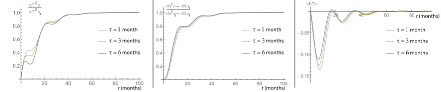
Figure 3.Evolution of the variance ofT(left),h(center) and of the cross-correlation betweenTandh, obtained from Equation (20b) with theAiandBicoefficients given by Equations (A7)–(A14), in the

case where 1/λ=12 month andϕ(t) =exp(−t/τ), for different values ofτ. Solid line:τ=6 months;

dashed line:τ=3 months; dotted line:τ=1 month. Curves for differentτvalues are very similar.

The results of this section allow us to get two main important conclusions:

1. analyzing only the first and second moments/cumulants/cross-correlation functions of the observations data, we cannot identify/detect the (possible) nonlinearity due to the interaction with the atmosphere, in the ENSO system;

2. comparing the first and second moments/cumulants/cross-correlation functions, we obtain from the FPE of Equation (18) with observations, it would be really hard to determine how small the time scaleτof decaying of the correlation function of the effective noise perturbing the ROM is. On the other hand, as has been shown in [17], also forτ → 0, the FPE of Equation (18) well accounts for the non-Gaussianity of the ENSO statistics. Thus, for the sake of simplicity, from now on, we shall use the FPE of Equation (17), which is the white noise limit of Equation (18), even if we are aware of the fact that the time scale separation between the dynamics of the averaged ROM and that of the fast atmosphere is not so “extreme”.

In the next subsection, we shall analyze Point 1 in detail.

6.2. The Covariance Matrix of the ROM and the Comparison with the ENSO Data

To this end, we write again the first equations for the time evolution of the first two moments, using the FPE Equation (17) (we also use the shifth→h+βD/ωto ensure that the mean value of the thermocline depth anomaly is zero):

˙

hhi=−ωhTi ˙

hTi=ωhhi −(λ−β2D)hTi ∼ωhhi −λhTi (23a)

˙

hh2_i=−2ωhhTi

˙

hhTi=ωhh2i −(λ−β2D)hhTi −ωhT2i ∼ωhh2i −λhhTi −ωhT2i

˙

hT2_{i=2ωhhTi −2(λ−2β}2_D)hT2_i+4

βDhTi+2D

∼2ωhhTi −2λhT2i+4βDhTi+2D. (23b) For the sake of simplicity, in the above equations, we have explicitly made the approximation of neglecting the terms proportional toβ2D, assuming thate 1 andβ 1. The validity of this assumption will be shown later. In any case, these approximations could be weakened without affecting the derivation below. From the above equations, we get the following stationary first and second moments:

hhis =hTis=0

hh2is =hT2is ∼ D

λ. (24)

The values of the ratioD/λcan be obtained from the observations with a very good accuracy. According to Equation (24),D/λcan be inferred from the varianceσ2=hT2isof the Niño 3 time series,

leading toD/λ∼0.8 (we recall thatD≡e2hξ2iτis the “standard” diffusion coefficient). For the other coefficients in the FPE of Equation (17), we focus our attention on the elements of the covariance matrix hx(t)y(0)is, where “x” and “y” can be eitherhorT. We note that by definition, we have:

hx(t)y(0)is=h

eL+FPEt_x

yis (25)

whereL+_FPEis the adjoint of the Liouvillian defined by the FPE of Equation (17). Thus, the evolutions (eL+FPEth)and(eL

+

FPEtT)are solutions of the differential equations for the lowest order moments of Equation (23a). Because Equation (23a) is linear, the solutions will be linear combinations ofhandT:

eL+FPEt_h

=ah,h(t)h+ah,T(t)T

eL+FPEt_T

=aT,h(t)h+aT,T(t)T (26)

where:

ah,h(t) =e− λ 2u

cos(Ωu) + λ 2

sin(Ωu)

Ω

ah,T(t) =−e− λ

2u_ωsin(Ωu) Ω

aT,h(t) =−ah,T(t)

aT,T(t) =e− λ 2u

cos(Ωu)−λ 2

sin(Ωu)

Ω

Exploiting Equation (26), Equation (25) becomes:

hh(t)h(0)is =hh2isah,h(t)

hT(t)h(0)is =hh2isaT,h(t)

hh(t)T(0)is =hT2isah,T(t)

hT(t)T(0)is =hT2isaT,T(t)

, (28)

where (see Equation (24))hT2_i

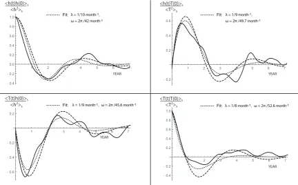
s =hh2is ∼D/λ∼0.8±0.3. In Figure4, we show the time evolution of the elements of the correlation matrix obtained from observations and the best fit obtained with Equation (27). This best fit yields values ofω = 2π /48 month−1andλ = 1/10 month−1, but the residuals of these fitting functions are quite large. For that, in the same figure, we also insert the plot of the same functions of Equation (27), but with the ROM coefficients given byω=2π/48 month−1and λ=1/12 month−1, which, as we shall see later, well agree also with other aspects of the data analysis.

1 2 3 4 5 6 7

-0.4

-0.2 0.0 0.2 0.4 0.6 0.8 1.0

1 2 3 4 5 6 7

-0.6

-0.4

-0.2 0.2

1 2 3 4 5 6 7

-0.2 0.2 0.4 0.6

1 2 3 4 5 6 7

-0.4

-0.2 0.2 0.4 0.6 0.8 1.0

Fit:

Fit: Fit:

YEAR YEAR

YEAR

YEAR

<h(t)h(0)>s

<h2_> s

<T(t)h(0)>s

<h2_> s

<h(t)T(0)>s

<T2_> s

<T(t)T(0)>s

<T2_> s

Fit: λ = 1/9 month-1,

ω = 2π /49.7 month-1 λ = 1/10 month-1,

ω = 2π /42 month-1

ω = 2π /45.6 month-1

λ = 1/9 month-1, λ = 1/8 month-1, ω = 2π /52.6 month-1

Figure 4.Correlation matrixhx(t)y(0)is/hy2is, where “x” and “y” can be eitherhorT. Solid line: from

the NOAA data (thehvalues are taken from [76] and refer to the anomalies of the Volume of Warm Water (WWV) in the basin 120◦E–80◦W, 5◦S–5◦N, in the time range from January 1982–December 2017). Dashed line, from the Fokker–Planck Equation (FPE) of the Recharge Oscillator Model (ROM), i.e., from Equations (27) and (28) in the case whereω =2π/48 month−1 andλ =1/12 month−1.

Dotted line: a fit with the same functions of Equations (27) and (28).

0.005 0.010 0.050 0.100 0.500 0.001

0.010 0.100 1 10

month-1

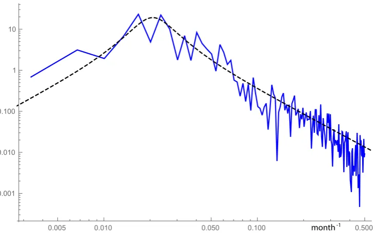
Figure 5. Solid blue line: periodogram of the Niño 3 data from NOAA evaluated averaging over non-overlapping partitions of length 300 months. Dashed black line: theoretical power spectrum of an ROM withω=2π/48 month−1,λ=1/10 month−1and additive white noise perturbation.

6.3. Signatures of a Nonlinear Perturbation: Skewed Stationary PDF and High Frequency of Strong Events As we have already noticed, if we focused on the first and second moments of the ENSO, we would not be able to estimate the value of the parameterβresponsible for the nonlinearity of the perturbed ROM of Equation (15) (or the FPE of Equation (17)). To infer the value of theβparameter, we have to focus our attention on the non-Gaussian character of the ENSO statistics; hence, we have to evaluate the stationary PDF of the FPE of Equation (17). Although this FPE is simplified with respect to the more general one (Equation (18)), the exact stationary PDF is not known. It has been shown in [17], using a reasonable ansatz, that it is possible to obtain the following analytic expression for the reduced stationary PDF of the soleTvariable (see also AppendixC):

ps(T) =βfµ

µ−2 1+βT

forT>−1/β

ps(T) =0 forT≤ −1/β, (29)

µ≡1+ λ

Dβ2, (30)

where the Gamma-like density function fµ(x)is defined as:

fµ(x)≡

1

(µ−2)Γ(µ−1)e

−x_xµ_{, (31)}

“heavy” tail of the stationary PDF, strongly depends on the value of theβparameter. The maximum of the stationary PDF is found atTmax =−2/(βµ)≈ −2βD/λ; for fixedD/λ, it is proportional toβ. The probability of strong negative values ofT(La Niña events) is largely reduced, and it is null for temperatures smaller than the thresholdTmin=−1/β.

This skewed stationary PDF forTfits well the data from observations (see Figure1) withβ=0.2 andD/λ=0.8 (µ=32.7). The value forD/λis in agreement with the range of values we have already obtained for the variance of the ROM; hence, from now on, we setD/λ=0.8 andβ=0.2.

From the FPE of Equation (17) and using the same ansatz that leads to the stationary PDF in Equations (29)–(31), it is also possible to obtain an analytical expression for the mean First Passage Time (FPT) for the ENSO events [77] and to compare these results with the observations. More precisely, we are interested in the average time we have to wait for the onset of a “strong” El Niño event, starting from a “neutral” initial condition defined as the case when the temperatureTihas a value in the range

−0.5 ≤ Ti ≤ 0.5. As depicted in Figure6, “strong” El Niño events are identified by the criterion

T > 1.5. Thus, the FPT is defined as the time δt(Ti|Ttg)whenT(t)first crosses a given targetTtg,

starting from the initial valueTi(see Figure7). However, ifT(t)is a stochastic process, repeating many

times the same “experiment” should lead to different values forδt(Ti|Ttg), so that the FPT itself is a

stochastic process, with its own PDF. We indicate withtn(Ti|Ttg)thenthmoment of the PDF of the

FPT. Of course, the mean FPT is given byt1(Ti|Ttg). As we have shown in [77], we have:

t1(Ti|Ttg) = 





2 ps(T)

β 2λ

Mh1,−(µ−2),−_βµ_T−₊2₁

i

βT+1





 Ttg

Ti

, (32)

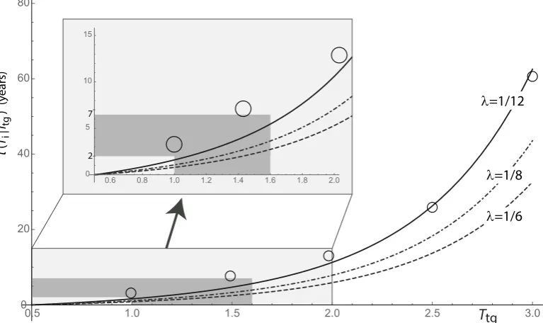
where{g(x)}b_a≡g(b)−g(a)andM[1,α,y]is the Kummers (generalized hypergeometric) function of the first kind with the first argument equal to one. We plot Equation (32) in Figure8to show the dependence of the mean FPT onTtgfor different values of theλparameter.

From this figure, we see thatλ=1/12 months−1, i.e., a value at the lower end of the expectedλ range, provides the best agreement between observational estimates and our analytic result for the mean FPT. Withλ=1/12 months−1, the mean FPT for intermediate target temperatures, obtained from Equation (32), is in the range of 2–7 years, in good agreement with the observed intervals between intermediate El Niño events. Apart from the inverse proportionality relationship with the relaxation coefficientλ, it is also clear that the average FPT has a strong sensitivity to the value of theβparameter (once the varianceσ2 ∼ D/λis kept fixed, theµparameter depends only onβas ∼1/β2). In Figure9, we compare the average FPT of Equation (32) with the values obtained through the numerical integration of the stochastic differential equation equivalent to the FPE of Equation (17) using β = 0.2. We can see that there is a good agreement between the analytical and numerical solutions. In the same figure, we also show the analytical solutions of the average FPT in the case of a pure additive perturbation (β=0, in which case, the reduced stationary PDF for theTvariable is Gaussian) and forβ=0.3. For weak to intermediate El Niño events (Ttg ≤1.5), the average FPT

depends weakly onβ. However, the sensitivity toβclearly emerges in the case of strong and very strong events. In particular, the purely additive forcing leads to average FPT that are many orders of magnitude larger than those obtained withβ=0.2 (note the logarithmic scale in the ordinate of the graph), while in the case ofβ=0.3, the FPTs are shorter at largeTtg.

strong or very strong El Niños, and the fact that this extrapolation fits well to the (few) available data is encouraging.

1 9 17 25 33 41 49 57 65 73 81 89 97 105 113 121 129 137 145 153 161 169 177 185 193 201 209 217 225 233 241 249 257 265 273 281 289 297 305 313 321 329 337 345 353 361 369 377 385 393 401 409 417 425 433 441 449 457 465 473 481 489 497 505 513 521 529 537 545 553 561 569 577 585 593 601 609 617 625 633 641 649 657 665 673 681 689 697 705 713 721 729 737 745 753 761 769 777 785 793 801

97-98 82-83

72-73

Weak Moderate Strong Very Strong Extremely Strong

Weak Moderate Strong Very Strong

SST Anomaly at NINO.3 (5S-5N, 150W-90W)

-2.5 -2 -1.5 -1 -0.5 0 0.5 1 1.52

2.5 3 3.5 4

δt

Figure 6.The month averaged Niño 3 data from January 1949–February 2016. Data are from the Tokyo Climate Center, WMO Regional Climate Centers (RCCs) [78]. In green, we highlight a segment of the time series to illustrate the First Passage Time (FPT)δt(Ti,Ttg)for a given target temperature anomaly Ttg(here,Ttg=1.5), starting from an initial neutral temperatureTi(−0.5≤Ti≤0.5). See also the text

and Figure7for details about the FPT.

-1.5 -1 -0.5 0 0.5 1 1.5 2

1 7 13 19 25 31 37 43 49 55 61 67 73 79 85 91 97 103 109 115 121 127 133 139 145 151 157 163 169 175 181 187 193 199 205 211

δt

t (months)

T

T_tg

Figure 7.The first passage timeδt(Ti,Ttg)for a target temperature anomaly ofTtg=1.5 is defined as

the first time the fluctuating temperatureT(t)crosses the thresholdTtg(1.5 in this case), starting from

an initial temperatureTi(that we will choose in the range−0.5≤Ti≤0.5, corresponding to neutral

1.0 1.5 2.0 2.5 3.0 20

40 60 80

0.6 0.8 1.0 1.2 1.4 1.6 1.8 2.0 5

10 15

0

λ=1/12

λ=1/8

λ=1/6

2 7

T

0 0.5

t

(

T |T

)

(y

ears)

i

tg

Figure 8.The mean FPT for different values of theλparameter, vs. the target temperature, obtained

using Equation (32), compared with observations (circles). The values ofβandµhave been fixed by

fitting the stationary PDF of Equations (29)–(31) to Niño 3 from [50]: β=0.2 andµ=32.7 (see the

text for details). Dashed line:λ = 1/6 month−1, dotted-dashed lineλ =1/8 month−1, solid line λ=1/12 month−1. In the inset, a zoom of the same graphs, where the gray background emphasizes

the range of 2–7 years and 1.0≤ T ≤1.6, corresponding to the typical recurring time interval for intermediate El Niño events. Notice how the curve obtained withλ=1/12 month−1falls better than

the others in this zone.

1.0 1.5 2.0 2.5 3.0 3.5

0.1 1 103

102

10 104

0.5

t

(

T |T

)

(y

ears)

i

tg

T

β=0

β=0.2

β=0.3

Figure 9. Semi-log plot of the average FPT as a function of the target temperatureTtg, for λ =

1/12 month−1andσ2=D/λ=0.8 (see the text for details). Thick and thin solid lines show analytical

solutions from Equation (32) withβ=0.2 andβ=0.3, respectively; while the thick dashed line is for

the caseβ=0, corresponding to the pure additive forcing of the ROM (in this case, the stationary PDF is

the Gaussian). Circles: the average FPT from Niño 3 data from NOAA [50]. Crosses: average FPT from numerical simulations of the Îto SDE corresponding to the FPE of Equation (17) [79]: dh=−ωTdt;

dT= (−ωh+Dβ)dt−(λ−Dβ2)Tdt+ √

6.4. Inferring the FPE Coefficients from Data

The results of the previous sections validate the FPE of Equation (17) with parametersω=2π /48 month−1,λ =1/12 month−1andD/λ= 0.8. However, at least in principle, there is a way to infer the transport coefficients of an FPE directly from data. For that purpose, let us rewrite the FPE of Equation (17) in the following way:

∂tσ(h,T;t) =

n

−∂hGh(h,T)−∂TGT(h,t) +∂2_TA(T)

o

σ(h,T;t), (33) where (as in Equation (23) we used the transformationh→h+βD/ωto eliminate the mean value of the thermocline depth anomaly):

A(T)≡D(1+βT)2 GT(h,T)≡ωh−(λ−Dβ2)T

Gh(h,T)≡ −ωT. (34)

It is well known that given the FPE of Equation (17), the drift and diffusion coefficients can be inferred using their statistical definitions as conditional first and second moments of the process increments [80–82]:

A(T) =1 2δlimt→0

1 δt

Z ∞

−∞(T−T

0₎2_P(h0_,T0_|h,T;δt)dh0_dT0 _(35a)

GT(h,T) =lim

δt→0

1 δt

Z ∞

−∞(T−T

0_)P(h0_,T0_|h,T;δt)dh0_dT0 _(35b)

Gh(h,T) =lim

δt→0 1 δt

Z ∞

−∞(h−h

0

)P(h0,T0|h,T;δt)dh0dT0, (35c)

in whichP(h0,T0|h,T;δt)is the conditional probability to go from(h,T)to(h0,T0)in an infinitesimal timeδt. From a practical viewpoint, the above expressions are obtained from the expectation values of the first (Equations (35b) and (35c)) and second (Equation (35a)) moments of the difference of two subsequent Niño 3 values, where the time step isδt=1 month. Because the duration of thehtime series is too short to obtain a reliable two-dimensional PDF (note that forh, we use the “proxy” given by the anomalies in the volume of Warm Water (WWV) in the basin 120◦E–80◦W, 5◦S–5◦N, in the time range from January 1982–December 2017, taken from [76]), we focus our attention only on the T variable, i.e., we work only with the observed Niño 3 index. This means that we disregard the drift coefficient of Equation (35c), and for eachTvalue, when we evaluate the expectation of the first and second moments of the process increments ofT, we automatically average overhat fixedT. This average over thehvariable does not affect the diffusion coefficient of Equation (35a), thus,

E[(T(t+δt)−T(t))2]

2δt = A(T) =D(1+βT)

2_{, (36)}

while for the drift coefficient of Equation (35b), we have:

E[T(t+δt)−T(t)]

δt =hGT(h,T)iT,s ≡ωhhiT,s−λT+α e

2

1β(1+βT)

∼ −(λ−Dβ2)T' −λT, (37) whereh...iT,s means the conditional stationary average at fixedT, and in the second line, we have

The functions in Equations (36) and (37)) correspond to the diffusion and drift coefficients, respectively, of the following reduced FPE for theTvariable:

∂tp(T;t) = n

(λ−Dβ2)∂TT+∂2_TD(1+βT)2

o

p(T;t), (38)

that is, the same FPE we would obtain directly by using the already cited ansatz introduced in [17], in the FPE of Equations (17)–(34). In Figure10, we see that from the Niño 3 data, the expectation value,

E[T(t+δt)−T(t)]looks as a linear function ofT, supporting again the view of a linear unperturbed

ROM, and the linear fit is very close to−λT withλ = 1/12 month−1, the same values we have obtained from the mean FPT analysis of the previous subsection.

Concerning the diffusion coefficient, evaluated as in Equation (35a), we see from Figure11that the expectation valueE[(T(t+δt)−T(t))2]/2 is compatible with the square dependence onT of

Equation (36), but the the uncertainty is large. This large uncertainty is due to the nonlinear nature ofA(T), which makes the fitting process strongly dependent on largeTvalues where the statistics is poor. The large value of theE[(T(t+δt)−T(t))2]/2 for large negativeT(∼ −2) suggests thatβcould be quite larger than 0.2 (leading to a diffusion term more symmetric with respect to zero compared with the caseβ=0.2); however, in this case, it would be necessary to add another noise term, additive and uncorrelated with the CAM one,to explain the other results so far presented. Actually, this is the perturbation already introduced in Equation (16), and the corresponding diffusion coefficient is shown in the same Figure11as a dashed green line. The case where an additional uncorrelated noise is added to the present perturbed ROM will be deeply analyzed in a forthcoming work.

- 2 -1 1 2 3

- 0.2

0.2 0.4 0.6 0.8 1.0

T

[

T

(

t+

δ

t

)

-T

(

t

)]

E

Figure 10. Dots: the expectation valueE[T(t+δt)−T(t)]whereδt =1 month, of the Niño 3 data

from NOAA [50]compared with the drift coefficienthGT(h,T)iT,s' −λT(see Equation (37)), in the

cases where the coefficientλis obtained as the the best fit to the data (dashed green line), from which λ=1/13.7 month−1, close to the case whereλ=1/12 month−1(solid red line) that corresponds to

-

3

-

2

-

1

1

2

3

0.05

0.10

0.15

0.20

0.25

E

[(

T

(

t+

δ

t

)

-T

(

t

)) ]

2

2

T

data from NOAA [50]. Solid red line: diffusion termA(T) =D(1+βT)2(see Equation (36)), where β =0.2 andD =σ2λ =0.07 month−1(see the text for details). Gray dashed line: the number of

observed events for each value ofT, scaled by a factor 1/160 in the vertical axes. The points for extreme events are not that close to the red line, but in these cases, the statistics is also really poor. Green dotted line, functionD(1+βT)2+D1, with the following figures obtained from the fit to the data with fit parametersβandD(D1=σ2λ−Dto ensure a fixed variance of the PDF):β=0.9,D=0.011 month−1

andD1=σ2λ−D=0.07 month−1−0.011 month−1=0.059 month−1.

7. Discussion and Conclusions

Starting from the fact that the ENSO statistics has some clear non- Gaussian features, in this paper, we use the results of some recent papers, and we analyze further the statistics of the ENSO, with the specific goal of discussing which non-linear dynamics might be responsible for them. Thus, as in [17], we work with the Fokker–Planck Equation (FPE) for the PDFof the ROM variables, but here aiming at the search for nonlinearities. In this simplified model, we consider two possible sources of nonlinearities: nonlinearity in the dynamics of the unperturbed ROM and a nonlinear (i.e., multiplicative) fast perturbation of the ROM.

Comparison with observations leads to the conclusion that a possibly nonlinear interaction between the internal ROM variables cannot be inherently the cause of the observed non-Gaussianity, which instead is well reproduced assuming a linear ROM with a nonlinear chaotic perturbation.

The hypothesis of nonlinear interaction between the unperturbed ROM and the fast forcing is strongly supported by the comparison between observations and theoretical results (stationary PDF and average FPT) for values ofTwhere the number of observation data is statistically relevant (weak and intermediate ENSO).

It is noticeable that extrapolating this result also for largeT, the heavy tail of the PDF leads to relatively short recurring times of strong ENSO, which still fit well to the few observations and that are orders of magnitude smaller than those we would have in the Gaussian case.

because nonlinearities become important in the largeTrange (rare events), where the statistics is rather poor (dashed line in Figure11).

We can conclude that the nonlinear interaction between the fast and slow modes of the ENSO gives a substantial contribution to the non-Gaussianity of the ENSO statistics. However, further work is necessary to better quantify the nonlinear nature of the perturbation, which is related to the nonlinear diffusion coefficient of the FPE. For example, from observations, we see that the expectation valueE[(T(t+δt)−T(t))2]/2, which should reproduce the functional dependence of the diffusion

coefficient with respect to theTvariable, is compatible with the CAM diffusion termA(T) =D(1+ βT)2of Equation (36) with a small beta (β∼0.2), but also with the case where there is another diffusion coefficientD1, in this case constant. In fact, it turns out that the sumD1+A(T)fits to the data, as

well as A(T)alone (see in Figure11), but with an increased value forβand a decreased value for D(the sumD+D1must be kept fixed to preserve the value of the variance). Thus, to be able to

define the actualD1andβvalues, we should increase the sample size used for the fitting process, for example using longer time series from century-long reanalysis products (CERA 20C,https:// www.ecmwf.int/en/forecasts/datasets/archive-datasets/reanalysis-datasets/cera-20c) and/or proxy data (networks of precipitation, tree-rings, corals and ice core records) that can help extend the time series back in time some hundreds of years [83]. Another point that deserves more investigation is the role of the weak nonlinearity in the interaction between the ROM variableshandT, under the current assumption of the nonlinear perturbation. In fact, in Section3, we have assumed a linear (i.e., additive) perturbation to show that the internal nonlinearities cannot be the cause of the observed non-Gaussianity of the Niño 3 PDF. However, how much does the internal nonlinearity affect the PDF in the case of a nonlinear interaction? This is not a trivial question because, as we have shown in this paper, the nonlinear interaction leads to a much slower decay of the PDF, with respect to the linear (i.e., additive) case, and the tails of the PDF are where the small nonlinear terms can emerge. These are all issues on which we are currently working.

Author Contributions:Conceptualization, Marco Bianucci (MB). Formal analysis, MB, Riccardo Mannella (RM) and Silvia Merlino (SM). Data, MB, RM, SM and Antonietta Capotondi (AC). Methodology MB, RM and AC. Validation, RM and AC. Writing—original draft, MB and SM. Writing—review and editing, MB, AC, RM and SM. Funding:This research received no external funding.

Conflicts of Interest:The authors declare no conflict of interest.

Appendix A Validation of the Linear Relationship between the Wind Stress andTE

Equation (4) is an assumption that agrees with observations, as shown in the following. The wind stress is considered proportional to the square of the wind velocity at 10 m from the sea surface, taken from [61]. FigureA1shows the equatorial zonal (i.e., averaged over 5◦ S–5◦N) wind velocity for different longitudes. We see that very close to the Americas’ coasts (81◦W), the direction of the wind flips from trade wind to westerly. This is due to the thermal gradient we have when we pass from the cold East Pacific Equatorial Ocean to the warm Central American lands. Thus, for the wind stress τsof Equation (4), we use the anomaly (i.e., 1948–2018 mean removed) of the equatorial zonal wind

stress averaged in the longitude interval 180◦W–120◦W. The fluctuating quantityτsis divided into

slow (τs,slow) and fast (τs,f ast) components. Theτs,slowdata are obtained from the one-year average of

τsdata, whileτs,f ast≡τs−τs,slow. Then:

(1) From FigureA2, we clearly see that the time behaviors ofτ_s,slow andT_E,slow are similar (of course, some lag remains between the wind stress, which is a a forcing term, and the ocean reaction);

(2) From FigureA3, we see that the plot of the cross-correlation betweenτs,slowandTE,slowvs. time

(in moths) is very similar to the plot of the autocorrelation ofTE,slow(notice the little time offset

of the same figure, we see that the average relationship betweenτs,slowandTE,slowis mainly

linear, with a small dispersion of the data around the linear fit (quantities are normalized by the standard deviation of the quantities from observations):

τs ≡τs,slow+τs,f ast=k TE+τs,f ast. (A1)

The above two arguments strongly support the hypothesis expressed by Equation (4).

1960 1970 1980 1990 2000 2010

- 8

- 6

- 4

- 2 2 4

81W

98W

140W

180W

U (m/s)

Figure A1.5N–5S averaged zonal wind for different longitudes. Data from NOAA [61].

Appendix B Very Short Review of the Projection Approach Applied to the ROM

In the present work, we study the same ROM considered in [17]; however, we do not use the FPE in Equations (3) and (4) of [17] because of a marginal mistake: a missing additive term in the FPE, which here we want to fix. Thus, for the reader’s convenience, in the following, we give a short summary of the projection procedure adapted to the present case.

The idea of this approach is to assume that the fast fluctuating forceξ(t)has a deterministic nature, namely that the ROM of Equation (15) is just a part of a set of equations describing a larger deterministic system:

˙

h=−ωT ˙

T=ωh−λT+e ξ(1+βT) ˙

ξ=F(ξ,π)

˙

π =Q(ξ,π). (A2)

Using the terminology of the projection approach [27,66,84], the ROM is viewed as the “system of interest” (or systema), while(ξ,π)represents the booster system (or “rest of the system” or systemb),

namely a set of general chaotic and fast variables, e.g., the MJO and WWB [85–89], which, perturbing the ROM, activate the El Niño/La Niña phenomena and which obey some unspecified equations of motion expressed by the generic functionsF(ξ,π)andQ(ξ,π). The value of the parametere determines the intensity of the perturbation to the ROM. Fore=0, the first two lines of Equation (A2) define the unperturbed system of interest (or unperturbed ROM).

We stress that we leave unspecified the exact expressions of the functionsF(ξ,π)andQ(ξ,π),

More generally, the interaction between the ROM and the booster should be bi-directional: the booster equation of motion should be affected by the dynamics of the ROM:F =F(ξ,π,eR(h,T)) andQ=Q(ξ,π,eR(h,T)). The functioneR(h,T)is the “reaction” force of the ROM variables on the MJO/WWB system. However, for the sake of simplicity, we shall consider hereaftereR(h,T) =0 as in [17]. The feedback term can be included following the general approach of [26,33]. The goal is to describe the statistics of the part of interest. We start from the following Langevin equation for the PDFρ(h,T,ξ,π;t)of the total system:

∂tρ(h,T,ξ,π;t) ={La+eLIξ+Lb}ρ(h,T,ξ,π;t) (A3)

where the unperturbed and perturbation Liouville operators are given by:

La =ω ∂hT−ω ∂Th+λ ∂TT

LI =−∂T(1+βT), (A4) respectively. In Equation (A3), we do not write the explicit expression of the Liouville operatorLbof

the booster because it is related to the unknown functionsF(ξ,π)andQ(ξ,π).

We are interested in obtaining a Fokker–Plank Equation (FPE) for the reduced (or marginal) PDF of the system of interest, given byσ(h,T;t) ≡ R ρ(h,T,ξ,π;t)dξdπ. Introducing the projection

operator, P· · · ≡ ℘b(ξ,π)R dξdπ· · ·, where ℘b is the stationary PDF of the booster, defined

by ℘_b(ξ,π) | Lb℘b(ξ,π) = 0, we have: σ(h,T;t) = 1/℘b(ξ,π)×Pρ(h,T,ξ,π;t). Following

the Zwanzig-like formal projection approach in the perturbation version of [64–66] to the lowest non-vanishing order on the coupling parametere, the time evolution ofσ(h,T;t)is governed by the following integro-differential equation:

∂tσ(h,T;t) =Laσ(x;t) +e2hξ2i_b

LI

Z ∞

0 duϕ(u)e

LauL

Ie−Lau

σ(h,T;t) (A5) In the above equation,ϕ(u)is the normalized auto-correlation function of the booster variableξ andhξ2ibis the variance ofξ(without any loss of generality, we assumedhξib=0). A very important

outcome of Equation (A5) is that we can group all the possible booster dynamical systems in different classes of equivalence, where all the boosters belonging to the same class give rise to the same statistical properties for a given system of interest. In fact, the FPE depends only on the booster autocorrelation functionhξ2ibϕ(u): different dynamical systems that share the same autocorrelation function belong to the same booster class of equivalence. Given Equation (A4), we can rewrite Equation (A5) as:

∂tσ(h,T;t) =

∂hωT−∂Tωh+λ ∂TT

+β e2hξ2i_bτ ∂T(1+βT) +e2hξ2ib∂T(1+βT) ×

Z ∞

0 duϕ

(u) 1+βTa(h,t;−u)eLau∂Te−Lau

σ(h,T;t), (A6) where we have used the identity