Vol.7 (2017) No. 1
ISSN: 2088-5334
Multi-Area Economic Dispatch Performance Using Swarm
Intelligence Technique Considering Voltage Stability
Mohd Khairuzzaman Mohd Zamani
#, Ismail Musirin
*, Saiful Izwan Suliman
#, Muhammad Murtadha
Othman
#, Mohd Fadhil Mohd Kamal
##
Faculty of Computer & Mathematical Sciences, Universiti Teknologi MARA, 40450 Shah Alam, Selangor, Malaysia E-mail: [email protected]
* Faculty of Electrical Engineering, Universiti Teknologi MARA, 40450 Shah Alam, Selangor, Malaysia
E-mail: [email protected], [email protected], [email protected], [email protected]
Abstract— Economic dispatch is one of the important issues in power system operation and planning. Economic dispatch requires reliable technique to achieve minimal cost; otherwise, a non-optimal solution may cause non-economic electricity generation to the utility. Single area economic dispatch does not make complete electricity generation of the whole system on the electrical transmission network. Thus, multi-area economic dispatch implementation leads to complete consideration for power transmission system. This paper presents multi-area economic dispatch performance using swarm intelligence technique. In this study, swarm intelligence technique, namely the particle swarm optimization technique (PSO) is employed for solving multi-area economic dispatch problems. The algorithm is tested on a 2-area 48-bus power system with different case studies. Variation in active power loading in achieving an optimal solution is also considered in this study. Several trials were taken into consideration to assess the consistency of results. Comparative studies were performed with respect to evolutionary programming (EP) and revealed that PSO yields better results as compared to the EP.
Keywords— particle swarm optimization technique; evolutionary programming; economic dispatch; optimization
I. INTRODUCTION
Most developing countries have experienced progressing demand on their power system network. This phenomenon has caused the power generation increments leading to the increase in generation cost. This has also affected the price of electricity [1]. Therefore, there is a demand to reduce the generation cost [2]. For this purpose, economic dispatch (ED) is introduced in response to this demand. Economic dispatch is defined as a process of determining the optimal combination of power generation to reduce the total generation cost while satisfying all the imposed constraints [3].
Traditionally, ED problems are solved by using Lambda-Delta iteration method. Unfortunately, the constraints imposed to the ED problem have caused it to be a highly nonlinear problem and the traditional method cannot cater the ED problem well [4], [5]. In order to overcome this limitation, various authors have proposed a different method to solve ED. Several optimization techniques have been proposed by many researchers. Among the popular
techniques are Artificial Immune System (AIS), Particle Swarm Optimization (PSO) and Evolutionary Programming (EP) [6]-[9]. All these proposed optimization algorithms are only tested on the single-area power system, hence proving that all these algorithms are capable of performing single area ED. However, the multi-area economic dispatch (MAED) problems received lesser attention as compared to single area ED [10]. There are various studies, which introduce result comparison between EP and other modified or improved optimization algorithm such as Improved Particle Swarm Optimization (IPSO) [11]. There is no direct comparison between EP and classical PSO has been made. Due to this, there is no definitive proof of which algorithm would provide the best solution for MAED problems. A generalized claim should not be made to declare a chosen optimization technique is always good to solve such problem. Normally, a chosen optimization technique performed excellently to solve a problem. Nevertheless, it also depends on the control variables involved in the optimization process and nature of the problem formulations.
comparative study between classical PSO and EP to determine which algorithm would provide a better solution for MAED problems. The proposed study incorporated the basics of MAED such as generation limits and maximum tie-line power transfer limit [12].
This paper presents economic dispatch performance using swarm intelligence technique. Particle Swarm Optimization (PSO) has been applied to solve economic dispatch problem and later be compared with respect to Evolutionary Programming (EP) technique. Results obtained revealed that PSO outperformed EP in terms of achieving lower optimal cost.
II. MATERIAL AND METHOD
A. Problem Formulation
The main objective of economic dispatch (ED) is to ensure minimal cost in power delivery to the consumer. The aim of this study is to test 2 algorithms namely PSO and EP to solve multi-area economic dispatch problem. The objective of MAED is to determine the optimum generation value which will impose the lowest generation cost while satisfying the load demand and other constraints. Hence, the objective function is given by:-
∑∑
= ==
N j gij ij M iP
C
CT
1 1)
(
)
min(
(1)where CT is defined as the total generation cost of all
generating units. Cij (Pgij) is defined as the generation cost of ith generation unit at jth area and it is a function of the power
generated by ith generation unit at jth area, Pgij.
Mathematically, it is defined as
)
/
($
)
(
P
a
P
2P
h
C
ij gij=
ij gij+
β
ij gij+
γ
ij (2) where αij, βij, and γij are the cost coefficients of ith generationunits at jth area.
To satisfy the load demand, the total power generated by all generation units should cater the total real power demand
Pd and the total power loss in the system Pl. Mathematically,
it is represented as
l d M
i
gi
P
P
P
=
+
∑
=1(3)
However, there are some constraints imposed in solving the MAED problems. The first constraint is the range of operation of a generating unit. For any generation unit, it should operate within its minimum and maximum allowable power generation. It is expressed as:-
max min
gij gij
gij
P
P
P
≤
≤
(4)The next constraint is the maximum power transfer across each line. The power to be transferred through each tie-line from jth area to mth area PTjm should not exceed the
maximum specified [13].
max min
Tjm Tjm
Tjm
P
P
P
≤
≤
(5)There is a constraint exists in multi-area economic dispatch, which is known as area power balance constraint. This constraint requires all the generation units in jth area to generate enough power to cater the load demand in the area
PDj and the power, which will flow through the tie-line from jth area to mth area PTjm including the power losses at the
tie-line PTljm [14]. Mathematically, this constraint is represented
as follows:-
(
)
∑
∑
=+
+
=
M i N j Tljm Tjm Dj Gij TP
P
P
P
1 (6)where M is the number of generation units and NT is the
number of tie-lines from jth area to mth area.
B. Particle Swarm Optimization
Particle Swarm Optimization (PSO) was developed by [15]. It simulated the movement of organisms of bird flocks or fish schools. In PSO, particles are made up of 2 parameters which are position and velocity. The particle’s position represents the objective variables, while the particle velocity represents the step size of the particles for its next iteration [16].
The optimization process starts with the generation of random particles. The particles are “flown” around the problem space to search for a global optimum point. During the travel of the particles, 2 best values will be recorded, which is Pbest and Gbest. Pbest will record the particles with the best optimum point for the iteration and Gbest will record the particles with the best optimum point in the whole process. In PSO, optimum solutions are found by changing the velocity and position of the particles with respect to Pbest and Gbest in the current problem space. The process of PSO is summarized as follows:
• The initialization process is done by generating random numbers to represent the particles in the problem space with respect to all constraints imposed to the algorithm. PSO parameters are also set at this stage.
• At this stage, the fitness values of the generated particles are evaluated. Pbest and Gbest are also initialized at this stage.
• During this stage, the velocity and position of the particles are updated. This update will represent the travel of the particles to the best optimum point. Velocity is updated by using Equation (7) and position is updated by using Equation (8) as stated as follows:
( )
t
+
=
v
( )
t
+
c
×
(
Pbest
−
x
( )
t
)
+
v
ij1
ω
ij 1ε
ij ijc
2ε
×
(
Gbest
i−
x
ij( )
t
)
(7)( )
t
+
1
=
x
( )
t
+
v
( )
t
+
1
x
ij ij ij (8)• During this stage, Pbest and Gbest are updated.
C. Evolutionary Programming
Evolutionary Programming (EP) is a stochastic optimization technique based on search algorithm, which is developed by [17]. The goal of the algorithm is to achieve intelligence through simulation of evolution. This intelligence is defined by Fogel as the capability of the system to adapt its behavior to meet its goals in a range of environments, clarifying how simulated evolution can be used as a basis to achieve the goal [18].
EP seeks for the optimal solution of an optimization problem by evolving a population of candidate solutions over a number of iterations [19]. The candidates, which is known as the parent will be used to generate a new population of candidates, which is known as the offspring via mutation process. In this study, the parent is mutated by using a Gaussian distributed mutation process [20]. The parent and offspring are then combined and will be competing with each other. The survived candidates will be selected to be the parent for the next iteration. The process of the EP is summarized as follows:
• Initialization. Random numbers are generated to represent the individuals of the EP.
• Fitness 1 calculation. The fitness value of the parent is evaluated.
• Mutation process. The parent is mutated using the Gaussian distribution mutation technique. The mutation technique is mathematically represented as
(
)
−
+
=
max min max
,
,
0
,
'
f
f
x
x
N
x
x
ij j
j i j
i
β
(9)where β is the step size, xi,j is the parent, xj min and xj max is
the minimum and maximum value of parent, f1 is the fitness
value of the parent and fmax is the maximum fitness value.
• Fitness 2 calculation. The fitness value of the offspring is evaluated.
• Combination process. The parent and the offspring are combined together.
• Selection process. The parent and the offspring are competing with each other and the survivor is selected by using Elitism method.
• Convergence test. If the iteration does not satisfy the convergence criteria, then go to step 2. Else, terminate the process.
D. Page Layout
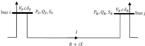
Fast voltage stability index is an instrument used to evaluate the stability of a particular stability through the FVSI value of the line. This method is developed by Musirin et al. In this study, the value of fast voltage stability index is used to observe the effect of variation of the output power of the generation units. In order to calculate the value of FVSI, 2 buses connected with a transmission line is depicted as in Fig. 1.
Fig. 1 Representation of 2-bus system for FVSI calculation By taking bus i as the sending bus and bus j as the receiving bus, the FVSI value of a transmission line is calculated using the formula as follows:
ij i
j ij ij
X
V
Q
Z
FVSI
=
4
2 (10)where Zij is the magnitude of the impedance of transmission
line connecting bus i and bus j, Qj is the reactive power at
the receiving end bus, Vi is the sending end bus voltage [22],
[23] and Xij is the magnitude of the reactance of the
transmission line connecting bus i and bus j. According to [21], FVSI values approaching the value of 1.00 indicates the instability of the line. Therefore, the lower value of FVSI indicates that the line is more stable.
III.RESULTS AND DISCUSSION
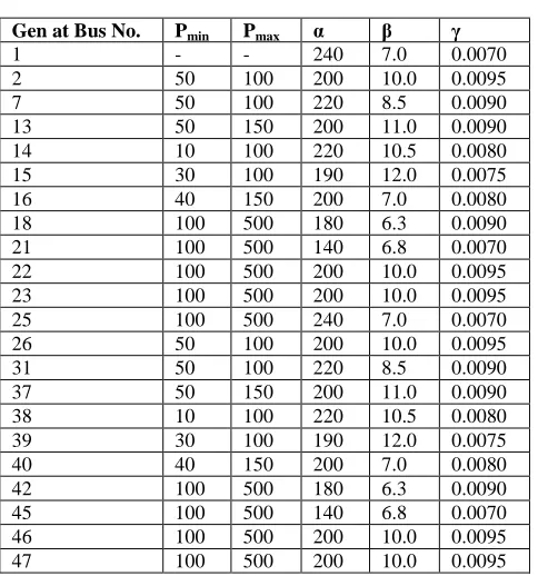
A comparative study is done between PSO and EP by solving multi-area economic dispatch problem. Both algorithms are tested on a 2-area 48-bus power system. The power system consists of 22 generating units in 2 areas, which are connected via 3 tie-lines. Table 1 tabulates the maximum and minimum limits of each generator in the system and their cost coefficient, while Fig. 1 illustrates the power system used in this study. Table 2 tabulates the load data of the power system used in this study.
Number of particles, N : N=20 Acceleration coefficients, c1 and c2 : c1=c2 = 2
Maximum velocity, vmax : vmax =100
Minimum velocity, vmin : vmin =−vmax
Inertia weight, ω : ω=1
The parameters set for EP are listed as follows
Number of candidates, N : N=20
TABLEI DATA OF GENERATION UNITS
Gen at Bus No. Pmin Pmax α β γ
1 - - 240 7.0 0.0070
2 50 100 200 10.0 0.0095
7 50 100 220 8.5 0.0090
13 50 150 200 11.0 0.0090
14 10 100 220 10.5 0.0080
15 30 100 190 12.0 0.0075
16 40 150 200 7.0 0.0080
18 100 500 180 6.3 0.0090
21 100 500 140 6.8 0.0070
22 100 500 200 10.0 0.0095
23 100 500 200 10.0 0.0095
25 100 500 240 7.0 0.0070
26 50 100 200 10.0 0.0095
31 50 100 220 8.5 0.0090
37 50 150 200 11.0 0.0090
38 10 100 220 10.5 0.0080
39 30 100 190 12.0 0.0075
40 40 150 200 7.0 0.0080
42 100 500 180 6.3 0.0090
45 100 500 140 6.8 0.0070
46 100 500 200 10.0 0.0095
47 100 500 200 10.0 0.0095
In order to test the algorithms, the result of the study is divided into 4 case studies which are:
Case 1 : Base case. The power system is operating at normal condition.
Case 2 : Contingency case. This condition simulates a contingency case where 1 of the tie-line is disconnected, which leaving the power system with only 2 tie-lines.
Case 3 : Generator outage case. In this condition, a generation unit at bus 23 area 1 is shut down hence reducing the total number of generation units by 1.
Case 4 : Load increment case. In this condition, the real power load at bus 8 area 1 is increased gradually from 0MW up to 450MW with 50MW steps.
TABLEII
LOAD DATA OF THE POWER SYSTEM
Area 1 Area 2
Bus No.
Real Power Load, (MW)
Reactive Power Load, (MW)
Bus No.
Real Power Load, (MW)
Reactive Power Load, (MW)
1 196.2 40.0 25 196.2 40.0
2 71.8 14.8 26 71.8 14.8
3 133.2 27.4 27 133.2 27.4
4 54.8 11.1 28 54.8 11.1
5 52.6 10.4 29 52.6 10.4
6 100.7 20.7 30 100.7 20.7
7 92.5 18.5 31 92.5 18.5
8 126.6 25.9 32 126.6 25.9
9 129.5 26.6 33 129.5 26.6
10 143.3 29.6 34 143.3 29.6
13 79.9 16.3 37 79.9 16.3
14 143.6 28.9 38 143.6 28.9
15 234.7 47.3 39 234.7 47.3
16 74.0 14.8 40 74.0 14.8
18 246.5 50.3 42 246.5 50.3
19 134.0 27.4 43 134.0 27.4
20 94.8 19.2 44 94.8 19.2
In case 1, 2 and 3, both algorithms will undergo the simulation process where both algorithms will be run for 5 times. Then, the average value of the results is taken. The algorithms are then compared based on the obtained values. For case 3, load increment condition is considered.
A. Case 1: Normal Condition
In this condition, the power system is operating at its normal condition. MAED problems are solved by using PSO and EP. Table 2 indicates the generation cost obtained by each algorithm after optimization process. It can be seen that both algorithms are capable of determining the best generation cost with PSO imposing a lower generation cost compared to the EP.
TABLEIII
GENERATION COST OBTAINED DURING NORMAL CONDITION
Attempt Generation Cost by Using PSO ($/h)
Generation Cost by Using EP ($/h)
1 48539.55 49361.88
2 48702.50 49815.83
3 48223.65 49585.27
4 48271.74 49585.27
5 48296.99 49585.27
Average 48406.89 49586.70
From Table 4 and Table 5, it can be observed that after optimization process has been executed, the FVSI values of all tie-lines has been reduced. PSO has clocked lower FVSI values on best FVSI values for tie-lines and the best FVSI value for the whole system. However, EP has produced better results on the worst FVSI values of tie-lines and the whole system compared to PSO. Therefore, it can be concluded that the optimization process has reduced the value of FVSI, hence implying that the system stability has also been improved.
TABLEIV
RESULT OF FVSIVALUES OF THE TIE-LINES DURING NORMAL
CONDITION
Tie-Line (Sending Bus-Receiving Bus)
Pre-Optimized FVSI
Post-Optimized FVSI
PSO EP
23-41 0.1198 0.0026 0.0198
13-39 0.0780 0.1004 0.1084
7-27 0.0989 0.0618 0.0697
TABLEV
RESULT OF BEST AND WORST FVSIVALUES FOR THE WHOLE POWER
SYSTEM DURING NORMAL CONDITION
Parameter Pre-Optimized Post-Optimized
PSO EP
Best FVSI 0.00175 0.00002 0.00059 Worst FVSI 0.43489 0.47955 0.38840
B. Case 2: Contingency Case Condition
In this condition, the power system is in the contingency condition where one of the tie-line is disconnected hence reducing the power transfer capability through the tie-line. MAED problems are solved by using EP and PSO. Table 3 indicates the generation cost obtained by each algorithm after optimization process.
TABLEVI
GENERATION COST OBTAINED DURING CONTINGENCY CASE
Attempt Generation Cost by Using PSO ($/h)
Generation Cost by Using EP ($/h)
1 48325.48 49553.72
2 48285.26 50836.14
3 48088.59 49585.27
4 48518.97 49585.27
5 48399.91 49585.27
Average 48323.64 49829.13
In this case, it can be observed from Table 3 that both algorithms have successfully imposed a lower generation
cost with PSO providing the lowest generation cost as compared to the EP.
From Table 7 and Table 8, it can be observed that the FVSI value has been improved after the optimization process. PSO has been able to produce a lower value of best FVSI for the tie-lines and the whole system. However, EP has been able to produce lower worst FVSI value for the tie-lines compared to EP. Therefore, it can be concluded that the optimization process has also reduced the value of FVSI for tie-lines and the whole system, hence increasing the system stability.
TABLEVII
RESULT OF FVSIVALUES OF THE TIE-LINES DURING CONTINGENCY C Tie-Line
(Sending Bus-Receiving Bus)
Pre-Optimized FVSI
Post Optimized FVSI
PSO EP
23-41 0.11984 0.00006 0.01978
13-39 - - -
7-27 0.09891 0.04338 0.06966
TABLEVIII
RESULT OF BEST AND WORST FVSIVALUES FOR THE WHOLE POWER
SYSTEM DURING CONTINGENCY CONDITION
Parameter Pre-Optimized Post-Optimized
PSO EP
Best FVSI 0.00176 0.00005 0.00060 Worst FVSI 0.43490 0.38711 0.38841
C. Case 3: Generation Unit Outage Condition
During this condition, generation unit at bus 23 area 1 is removed from the system. This condition was intended to simulate the effect of a generation unit shutting down from a power system. MAED problems in this condition are solved by using EP and PSO.
TABLEIX
GENERATION COST OBTAINED DURING GENERATION UNIT OUTAGE
CONDITION
Attempt Generation Cost by Using PSO ($/h)
Generation Cost by Using EP ($/h)
1 49298.07 50658.99
2 48468.53 50658.99
3 50139.37 50658.99
4 48476.09 50658.99
5 48231.45 50658.99
Average 48922.70 50658.99
TABLEX
RESULTS OF FVSIVALUE OF TIE-LINES DURING GENERATION UNIT
OUTAGE CONDITION
Tie-Line (Sending Bus-Receiving Bus)
Pre-Optimized FVSI
Post Optimized FVSI
PSO EP
23-41 0.2068 0.0063 0.0194
13-39 0.0113 0.1023 0.1232
7-27 0.0885 0.0738 0.1074
TABLEXI
RESULT OF BEST AND WORST FVSIVALUES FOR THE WHOLE POWER
SYSTEM DURING GENERATION UNIT OUTAGE CONDITION
Parameter Pre-optimized Post-optimized
PSO EP
Best FVSI 0.001563 0.000018 0.00077 Worst FVSI 0.448154 0.394711 0.391945
D. Case 4: Load Increment Condition
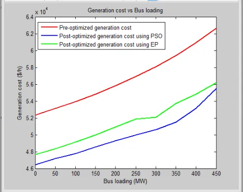
In this condition, the power system is working at its normal condition. The real power load at bus 8 is varied from 0MW up to 450MW with 50MW increment. At each loading, MAED problems are solved by using EP and PSO. Table 12 indicates the generation cost of the system obtained by using each algorithm at different loadings. Fig. 3 illustrates the data obtained from Table 12.
Fig. 3 Graphical representation of generation cost obtained load increment condition
From Table 12, it can be observed that with the increment of load at bus 8, both algorithms are capable of imposing a generation cost which is lower than the pre-optimized generation cost. The PSO algorithm yields the lower generation cost compared to EP at all loading conditions.
TABLEXII
GENERATION COST OBTAINED DURING LOAD INCREMENT CONDITION
Bus Loading (MW)
Generation Cost Before Optimization ($/h)
Generation Cost After Optimization Using PSO ($/h)
Generation Cost After Optimization Using EP ($/h)
0 52346.28 46473.39 47604.27
50 53118.57 47174.92 48364.93
100 53942.46 47778.04 49145.48
150 54829.91 48571.68 49987.01
200 55825.55 49284.23 50902.79
250 56907.19 49661.35 51882.38
300 58075.25 50617.12 52095.71
350 59405.52 51517.76 53723.15
400 60899.07 53137.22 54820.09
450 62675.69 55499.15 56205.48
IV.CONCLUSIONS
Multi-area economic dispatch is an important issue in power system optimization where it involves the solving of economic dispatch problems for multi-area power systems. From all case studies conducted in this paper, it can be concluded that both PSO and EP algorithms are capable of solving MAED problems while satisfying all constraints imposed to the problem with PSO yields better generation cost compared to the EP.
ACKNOWLEDGMENT
The authors would like to acknowledge The Institute of Research Management and Innovation (IRMI) UiTM, Shah Alam, Selangor, Malaysia for the financial support of this research. This research is supported by IRMI, UiTM under the LESTARI Research Grant Scheme with project code: 600-IRMI/MYRA 5/3/LESTARI (0024/2016).
REFERENCES
[1] J. Spínola, P. Faria, and Z. Vale, “Reconfiguration of distributed generation scheduling to increase demand response integration,” in
Proc. IEEE EEM’16, 2016, p. 1.
[2] X. Lai, L. Xie, Q. Xia, H. Zhong, and C. Kang, “Decentralized multi-area economic dispatch via dynamic multiplier-based Lagrangian relaxation,” IEEE Transactions on Power Systems, vol. 30, pp. 3225-3233, Nov. 2015.
[3] L. Coelho and V. Mariani, “Chaotic artificial immune approach applied to economic dispatch of electric energy using thermal units,”
Chaos, Solitons and Fractals, vol 40, pp. 2376-2383, Jun. 2009.
[4] N. Nahas and M. Abouheaf, “Novel heuristic solution for the non-convex economic dispatch problem,” in Proc. IEEE SSD’16, 2016, p. 742.
[5] H. M. Z. Iqbal and A. Shafique, “A hybrid evolutionary algorithm for economic load dispatch problem considering transmission losses and various operational constraints,” in Proc. IEEE ICISE’16, 2016, p. 202.
[6] S. Hemamalini and S. Simon, “Dynamic economic dispatch using artificial immune systems for units with valve-paint effect,”
International Journal of Electrical Power and Energy Systems, vol.
33, pp. 868-874, May 2011.
[7] Z. Gaing, “Constrained dynamic economic dispatch solution using particle swarm optimization,” IEEE Power Engineering Society
[8] M. Mahajan and S. Vadhera, “Economic load dispatch of different bus systems using particle swarm optimization,” in Proc. IEEE
PIC’12, 2012, p. 1.
[9] B. S. Rahimullah, E. Ramlan, and T. K. A. Rahman, “Evolutionary approach for solving economic dispatch in power system,” in Proc.
IEEE PECon’03, 2003, p. 32.
[10] U. Fragomeni, “Direct method to multi-area economic dispatch,” in
Proc. IEEE APCET’12, 2012, p. 1.
[11] V. Jadoun, N. Gupta, K. Niazi, A. Swarnkar, and R. Bansal, “Multi-area economic dispatch using improved particle swarm optimization,” Energy Procedia, vol. 75, pp. 1087-1092, Aug. 2015. [12] M. Ghasemi, J. Aghaei, E. Akbari, S. Ghavidel, and L. Li, “A
differential evolution particle swarm optimizer for various types of multi-area economic dispatch problems,” Energy, vol. 107, pp. 182-195, Jul. 2016.
[13] K. P. Nguyen, N. D. Dinh, and G. Fujita, “Multi-area economic dispatch using hybrid Cuckoo search algorithm,” in Proc. IEEE
UPEC’15, 2015, p. 1.
[14] V. Jadoun, N. Gupta, K. Niazi, and A. Swarnkar, “Multi-area economic dispatch with reserve sharing using dynamically controlled particle swarm optimization,” International Journal of Electrical
Power and Energy Systems, vol. 73, pp. 743-756, Dec. 2015.
[15] J. Kennedy and R. Eberhart, “Particle swarm optimization,” in Proc.
IEEE ICNN'95, 1995, p. 1942.
[16] A. Jaini, I. Musirin, N. Aminudin, M. Othman, and T. Rahman, “Particle swarm optimization (PSO) technique in economic power dispatch problems,” in Proc. IEEE PEOCO’10, 2010, p. 308.
[17] N. A. Aziz, S. Sulaiman, I. Musirin, and S. Shaari, “Assessment of evolutionary programming models for single-objective optimization,” in Proc. IEEE PEOCO’13, 2013, p. 304.
[18] L. Fang, “The new adaptive evolutionary programming,” in Proc.
IEEE ICMLC’10, 2010, p. 2341.
[19] G. Suganya, K. Balamurugan, and V. Dharmalingam, “Multi-objective evolutionary programming technique for economic/emission load dispatch,” in Proc. IEEE ICAESM’12, 2012, p. 269.
[20] S. K. Dash and C. K. Panda, “An evolutionary programming based neuro-fuzzy technique for multi-objective generation dispatch with non-smooth characteristic functions," in Proc. IEEE ICECS’15, 2015, p. 1663.
[21] I. Musirin and T. K. A. Rahman, “Novel fast voltage stability index (FVSI) for voltage stability analysis in power system,” in Proc. IEEE
SCOReD’02, 2002, p. 265.
[22] C. B. Risnidar, I. Daut, M. I. Yussof, E. Warman, S. Hasan, and I. Nisja, “Investigation of power factor on harmonic effect due to types of voltage source,” International Journal on Advanced Science,
Engineering and Information Technology, vol. 1, pp. 476-480, 2011.
[23] C. Risnidar, I. Daut, H. Syafruddin, E. Warman, and T. Kasim, “Investigation of harmonic characteristics in printer due to different types of voltage source,” International Journal on Advanced Science,