Bayesian Estimation Using MCMC Approach Based on Progressive First-Failure Censoring from Generalized Pareto Distribution

Published online August 30, 2013 (http://www.sciencepublishinggroup.com/j/ajtas) doi: 10.11648/j.ajtas.20130205.13

Bayesian estimation using MCMC approach based on

progressive first-failure censoring from generalized

Pareto distribution

Mohamed Abdul Wahab Mahmoud

1

, Ahmed Abo-Elmagd Soliman

2

, Ahmed Hamed Abd Ellah

3

,

Rashad Mohamed El-Sagheer

1, *

1

Mathematics Department, Faculty of Science, A1-Azhar University, Nasr-City 11884, Cairo, Egypt 2

Mathematics Department, Faculty of Science, Islamic University, Madinh, Saudi Arabia 3

Mathematics Department, Faculty of Science, Sohag University, Sohag 82524, Egypt

Email address:

[email protected] (Mohamed A. W. Mahmoud), [email protected] (Ahmed A. Soliman), [email protected] (Ahmed H. Abd Ellah), [email protected] (Rashad M. El-Sagheer)

To cite this article:

Mohamed Abdul Wahab Mahmoud, Ahmed Abo-Elmagd Soliman, Ahmed Hamed Abd Ellah, Rashad Mohamed El-Sagheer. Bayesian Estimation Using MCMC Approach Based on Progressive First-Failure Censoring from Generalized Pareto Distribution. American Journal of Theoretical and Applied Statistics. Vol. 2, No. 5, 2013, pp. 128-141. doi: 10.11648/j.ajtas.20130205.13

Abstract:

In this paper, based on a new type of censoring scheme called a progressive first-failure censored, the maximum likelihood (ML) and the Bayes estimators for the two unknown parameters of the Generalized Pareto (GP) distribution are derived. This type of censoring contains as special cases various types of censoring schemes used in the literature. A Bayesian approach using Markov Chain Monte Carlo (MCMC) method to generate from the posterior distributions and in turn computing the Bayes estimators are developed. Point estimation and confidence intervals based on maximum likelihood and bootstrap methods are also proposed. The approximate Bayes estimators have been obtained under the assumptions of informative and non-informative priors. A numerical example is provided to illustrate the proposed methods. Finally, the maximum likelihood and different Bayes estimators are compared via a Monte Carlo simulation study.

Keywords:

Generalized Pareto Distribution, Progressive First-Failure Censored Sample, Gibbs and Metropolis Sampler, Bayesian and Non-Bayesian Estimations, Bootstrap Methods

1. Introduction

Censoring is very common in life tests. There are several types of censored tests. One of the most common censored test is type II censoring. It is noted that one can use type II censoring for saving time and money. However, when the lifetimes of products are very high, the experimental time of a type II censoring life test can be still too long. (Johnson, 1964) described a life test in which the experimenter might decide to group the test units into several sets, each as an assembly of test units, and then run all the test units simultaneously until occurrence the first failure in each group. Such a censoring scheme is called first-failure censoring. (Jun, et.al 2006) discussed a sampling plan for a bearing manufacturer. The bearing test engineer decided to save test time by testing 50 bearings in sets of 10 each. The first-failure times from each group were observed. (Wu, et.al 2003; Wu, and Yu, 2005) obtained maximum likelihood estimates (MLEs), exact

progressive first-failure censored sampling, (Soliman, et.al 2011b) proposed a simulation-based approach to the study of coefficient of variation of Gompertz distribution under progressive first-failure censoring. Therefore, the purpose of this paper is to develops the Bayes estimates and Markov Chain Monte Carlo (MCMC) techniques to compute the credible intervals and bootstrap confidence intervals of the unknown parameters of Lomax distribution under the progressive first-failure censoring plan.

A random variable X is said to have generalized Pareto (GP) distribution, if its probability density function (pdf) is given by

( )

(1 / 1)

, ,

1

1 x ,

f

ζ

ζ µ σ

µ ζ

σ σ

− + −

 

=  + 

 

where µ ζ ∈, R and σ∈(0,+∞) . For convenience, we reparametrized this distribution by defining

/ ,1/

σ ζ β ζ α= = andµ=0. Therefore,

( 1)

( )

(

)

,

0, ,

0.

f x

=

αβ

α

x

+

β

− +α

x

>

α β

>

(1) The cumulative distribution function (cdf) is defined by

( ) 1

(

) ,

0, ,

0.

F x

= −

β

α

x

+

β

−α

x

>

α β

>

(2) Here

α

and

β

are the shape and scale parameters, respectively. It is also well known that this distribution has decreasing failure rate property. This distribution is also known as Pareto distribution of type II or Lomax distribution. This distribution has been shown to be useful for modeling and analyzing the life time data in medical and biological sciences, engineering, etc. So, it has been received the greatest attention from theoretical and applied statisticians primarily due to its use in reliability and life testing studies. Many statistical methods have been developed for this distribution, for a review of Pareto distribution of type II or Lomax distribution see (Chahkandi, and Ganjali, 2009; Lomax, 1954). For its applications as lifetime distribution and extensions, we refer to (Marshall, and Olkin, 2007). (Bryson, 1974) has argued that Pareto distribution of type II provide a very good alternative to common lifetime distributions like exponential, Weibull, or gamma distributions when the experimenter presumes that the population distribution may be heavy-tailed. Details on Pareto distributions as well as areas of application can be found in (Arnold, 1983; Habibullh, and Ahsanullah, 2000; Upadhyay, and Peshwani, 2003; Abd Ellah, 2003 and 2006). A great deal of research has been done on estimating the parameters of Pareto distribution of type II or Lomax using both classical and Bayesian techniques.

The rest of this paper is organized as follows. In Section 2, we describe the formulation of a progressive first--failure censoring scheme as described by (Wu, and Kuş, 2009). Estimation of the parameters is given in Section 3. In this section, the ML estimators of the parameters, approximate confidence intervals and bootstrap confidence intervals are

presented. We cover Bayes estimates and construction of credible intervals using the MCMC techniques in Section 4. A numerical examples are presented in Section 5 for illustration. In Section 6 we provide some simulation results in order to give an assessment of the performance of the different estimation method.

2. A Progressive First-Failure Censoring

Scheme

In this section, first-failure censoring is combined with progressive censoring as in (Wu, and Kuş, 2009). Suppose that

n

independent groups with

k

items within each group are put in a life test,

R

₁groups and the group in which the first failure is observed are randomly removed from the test as soon as the first failure (say

x

_{1: : :}R_{m n k} ) has occurred,

2

R

groups and the group in which the second failure is observed are randomly removed from the test as soon as the second failure (say

x

_{2: : :}R_{m n k}

) has occurred, and finally

(

)

m

R

m

≤

n

groups and the group in which the

m

−

th

failure is observed are randomly removed from the test as soon as the

m

−

th

failure (say

x

_{m m n k}R_{: : :} ) has occurred. The

x

_{1: : :}R_{m n k}

<

x

_{2: : :}R_{m n k}

< <

...

x

_{m m n k}R_{: : :} are called progressively first-failure censored order statistics with the progressive censoring scheme R. It is clear that

1 2

...

m

n

= +

m

R

+

R

+ +

R

. If the failure times of the

n k

×

items originally in the test are from a continuous population with distribution function

F x

( )

and probability density function

f x

( )

, the joint probability density function for

x

1: : :m n k

,

R

2: : :m n k

,...,

x

R

x

m m n k: : :

R

is given by

1, 2,..., 1: : : 2: : : : : :

( 1) 1 : : : : : :

1

(

,

,...,

)

(

)(1

(

))

j

m m n k m n k m m n k

m

k m

j m n k j m n k

j

f

x

x

x

A k

f x

F x

+ −

=

=

−

∏

R R R

R

R R (3)

1: : : 2: : : : : :

0

<

x

R_{m n k}

<

x

R_{m n k}

< <

...

x

_{m m n k}R

< ∞

,

(4) where

1 1 2

1 2 1

(

1)(

1)...

(

...

_m

1).

A

n n

R

n

R

R

n

R

R

R

₋

m

=

−

−

−

−

−

−

−

−

− +

(5)

There are four special cases:

case if

k

=

1

and

R

=

(0,..., 0)

, then n = m which corresponds to the complete sample. The last one if

1

k

=

and

R

=

(0,...,

n

−

m

)

, then the type II censored order statistics are obtained. Also, it can be seen that the progressive first-failure censored order statistics

X

R_1;m,n,k

,

X

R_2;m,n,k

, . . . ,

X

_mR_{;m,n,k can be viewed as a} progressively type II censored sample from apopulation with distribution function

1 (1

− −

F x

( ))

k.

3. Estimation of the Parameters

In this section, we estimate

α

and

β

,

by considering the maximum likelihood and we compute the observed Fisher information based on the likelihood equations. These will enable us to develop pivotal quantities based on the limiting normal distribution, the resulting pivotal quantities can be used to develop interval estimates also, we construct the bootstrap confidence interval.

3.1. Maximum-Likelihood (ML) Estimation

Let

x

_{i m n k}R_{: : :} ,

i

=

1, 2,...,

m

, be the progressively first-failure censored order statistics from GP(

α β

,

) the distribution of reparametrized Generalized Pareto (GP) distribution, with censoring scheme

R

. from (3), the likelihood function is given by

( ( 1 ) 1) ( ( 1 ) 1)

1

( | , )

( ) ,

i i

m m m m

k R k R

i i

d ata A k

x

α

α α

α β

α β

β

+ −

β

− + +

= = +

∏

ℓ (6)

where

A

is defined in (5) and

x

i is used instead of

: : :

i m n k

x

R . The log-likelihood function may then be written as

1

1

( | , ) log log log

( ( 1) 1) log( )

( 1) log . m i i i m i i

L data A m k m

k R x

k R

α β

α

α

β

α

β

= = = + + − + + + + +

∑

∑

(7)

Upon differentiating (7) with respect to

α

,

and

β

, and equating each result to zero, two equations must be simultaneously satisfied to obtain MLE of

⌢

α

and

⌢

β

, The maximum likelihood equations of

α

,

and

β

can be obtained as the solution of

1

1

(

| , )

(

1) log

(

1) log(

),

m i i m i i i

L data

m

k R

k R

x

α β

_β

α

α

β

= =

∂

₌

₊

₊

∂

−

+

+

∑

∑

(8) and 1 1 ( 1) ( | , )

( ( 1) 1)

. ( ) m i i m i i i k R L data k R x

α

α β

β

β

α

β

= = + ∂ ₌ ∂ + + − +

∑

∑

(9)

Solving ∂L data( _∂α| , )α β

=

0

for

α

gives, from (8)

⌢ ⌢ ⌢ 1 1 1

( 1) log( )

. ( 1) log

m i i i m i i

k R x

m k R

β

α

β

− = =   + +     = _{ } − +    

∑

∑

(10)

By using (10) in (9) we obtain ⌢

⌢

⌢

⌢

1 1

( 1) ( ( 1) 1)

0.

( )

m m

i i

i i i

k R k R

x

α

α

β

β

= = + ₋ + + ₌ +

∑

∑

(11)

Since (11) cannot be solved analytically some numerical methods such as Newtons method must be employed.to solve (11) and get the MLE,

⌢

,

β

and hence

⌢

α

, by using Equation (10).

3.2. Approximate Interval Estimation

The asymptotic variances and covariances of the MLE for parameters

α

,

and

β

are given by elements of the inverse of the Fisher information matrix

2

; ,

1, 2.

ij

L

E

i j

α β



_∂



=



−



=

∂ ∂





I

(12)

Unfortunately, the exact mathematical expressions for the above expectations are very difficult to obtain. Therefore, we give the approximate (observed) asymptotic varaince-covariance matrix for the MLE, which is obtained by dropping the expectation operator E

⌢ ⌢

⌢

⌢ ⌢

⌢ ⌢

⌢

1 2 2 2 2 2 2 ( , )

var( )

cov( , )

,

cov( , )

var( )

L

L

L

L

α β

α

α β

α

α β

β α

β

β α

β

2 2

1 1

( 1) ( 1)

,

( )

m m

i i

i i i

L L

k R k R

x

α β β α

β β = = ∂ ₌ ∂ ∂ ∂ ∂ ∂ + + = − +

∑

∑

(14) 2 2 2 1 2 1

( ( 1) 1)

( ) ( 1) . m i i i m i i k R L x k R α β β α β = = + + ∂ ₌ ∂ + + −

∑

∑

(15)

The asymptotic normality of the MLE can be used to compute the approximate confidence intervals for parameters

α

,

and

β

.

Therefore,

(1

−

γ

)100%

confidence intervals for parameters

α

,

and

β

.become

⌢ ⌢

⌢ ⌢

/ 2

/ 2

var( ) and var( ), Z Z γ γ α α β β ±

± (16) where Z_{γ/ 2} is the percentile of the standard normal distribution with right-tail probability γ/ 2 .

3.3. Bootstrap Confidence Intervals

In this subsection, we propose to use confidence intervals based on the parameteric bootstrap methods (i) percentile bootstrap method (Boot-p) based on the idea of (Efron, 1982). (ii) bootstrap-t method (Boot-t) based on the idea of (Hall, 1988). The algorithms for estimating the confidenc eintervals using both methods are illustrated as follows

3.3.1. Percentile Bootstrap Method

1)From the original data

x

≡

x

_{1: : :}R_{m n k}

,

2: : :m n k

,...,

x

R

: : :

m m n k

x

R compute the ML estimates of the parameters

⌢

α

and

⌢

β

by solving the nonlinear equations (10) and (11).

2)Use

⌢

α

and

⌢

β

to generate a bootstrap sample

x

∗

with the same values of

R m i

i

,

; (

=

1, 2,..,

m

)

using algorithm presented in (Balakrishnan, and Sandhu, 1995).

3)As in step 1, based on

x

∗ compute the bootstrap sample estimates of

α

and

β

,

say

⌢

α

∗ and

⌢

.

β

∗

4)Repeat steps 2-3

N

times representing

N

bootstrap MLE's of

( , )

α β

based on

N

different bootstrap samples.

5)Arrange all

⌢

s

α

∗′ and

⌢

,

s

β

∗′ in an ascending order to obtain the bootstrap sample (

ϕ

_l[1]

,

ϕ

_l[2]

,

...,

ϕ

_l[N]

),

1, 2

l

=

(where

⌢

⌢

1

,

2

).

ϕ α ϕ

≡

∗

≡

β

∗

Let

G z

( )

=

P

(

ϕ

_l

≤

z

)

be the cumulative distribution function of

ϕ

₁

.

Define

ϕ

_lboot

=

G

−1

( )

z

for given

z

.

The approximate bootstrap

100(1

−

γ

)%

confidence interval of

ϕ

_l is given by

1

[

( ),

(

)].

2

2

lboot lboot

γ

γ

ϕ

ϕ

−

3.3.2. Bootstrap-t Method

1)From the original data

x

≡

x

_{1: : :}R_{m n k}

,

x

_{2: : :}R_{m n k}

,...,

: : :

m m n k

x

R compute the ML estimates of the parameters

⌢

α

and

⌢

β

by solving the nonlinear Equations (10) and (11).

2)Using

⌢

α

and

⌢

β

generate abootstrap sample

1 2

{

x

∗

,

x

∗

,...,

x

_n∗

}.

Based on

{

x

₁∗

,

x

₂∗

,...,

x

_n∗

}

compute the bootstrap estimate of

α

and

β

using

(10

) and (

11)

, say

⌢

α

∗ and

⌢

β

∗ and following statistics ⌢ ⌢ ⌢ ⌢ ⌢ ⌢ 1 2 ( ) ( ) , ( ) ( ) n n T T

V ar V ar

α α

β

β

α

β

∗ ∗ ∗ ∗ ∗ ∗ − − = = where

⌢

(

)

V ar

α

∗ and

⌢

(

)

V ar

β

∗ are obtained using the Fisher information matrix.

3)Repeat step 2, N boot times.

4)For the

T

₁∗ and

T

₂∗ values obtained in step2, determine the upper and lower bounds of the

100(1

−

γ

)%

confidence interval of

α

and

β

as follows: let

H x

( )

=

P T

(

_i∗

≤

x

),

i

=

1, 2

be the cumulative distribution function of

T

₁∗ and

T

₂∗ . For a given

x

, define

⌢

⌢

⌢

⌢

⌢

⌢

1/ 2 1

1/ 2 1

( )

( )

( ),

( )

( )

( ).

Boot t

Boot t

x

n

V ar

H

x

x

n

V ar

H

x

α

α

α

β

β

β

− − − − − −

= +

= +

Here also,

⌢

( )

V ar

α

and

⌢

( )

V ar

β

can be computed as same as computing the

⌢

(

)

V ar

α

∗ and

⌢

(

)

V ar

β

∗ . The approximate

100(1

−

γ

)%

confidence interval of

α

and

β

are given by

⌢

⌢

⌢

⌢

( ),

(1

) ,

2

2

( ),

(1

) .

2

2

Boot t Boot t

Boot t Boot t

4. Bayesian Estimation Using MCMC

In this section we describe how to obtain the Bayes estimates and the corresponding credible intervals of parameters

α

and

β

when both are unknown. For computing the Bayes estimates, we assume mainly a squared error loss (SEL) function. In some situations where we do not have sufficient prior information, we can use non-informative uniform distribution as the prior distribution. This is particularly true for our study. The non-informative uniform prior distribution can be used for parameters

α

and

β

. The joint posterior density will then be in proportion to the likelihood function. Here we consider the more important case when the shape parameter

α

and the scale parameter

β

have independent gamma priors with the pdfs

1 1

if 0

( | , ) ( ) ,

0 if 0.

a

a b

b e a b a

α α α π α α − −  > 

= Γ

 _≤  (17) and 1 2

if 0

( | , ) ( ) .

0 if 0. c

c d

d e

c d c

β β β π β β − −  > 

= Γ

 _≤



(18)

The likelihood function of the observed sample is same as (6) . Using the joint prior distribution of

α

and

β

, we obtain the joint distribution of the data,

α

, and

β

as

1 2

(

data

| , )

α β π α

×

( | , )

a b

×

π β

(

| , ).

c d

ℓ

₍₁₉₎

Based on (19), the joint posterior density of

α

and

β

given the data is

1 2

1 2

0 0

( , |

)

(

| , )

( | , )

( | , )

,

(

| , )

( | , )

( | , )

l

data

data

a b

c d

data

a b

c d d d

α β

α β π α

π β

α β π α

π β

α β

∞ ∞

=

×

×

×

×

∫ ∫

ℓ

ℓ

(20)

therefore, the Bayes estimate of any function of

α

and

β

say

g

( , )

α β

, under squared error loss function is

⌢

, | 1 2 0 0 1 2 0 0

( , )

( ( , ))

( , ) (

| , ) ( | , ) ( | , )

.

(

| , ) ( | , ) ( | , )

data

g

E

g

g

data

a b

c d d d

data

a b

c d d d

α β

α β

α β

α β

α β π α

π β

α β

α β π α

π β

α β

∞ ∞ ∞ ∞

=

∫ ∫

=

∫ ∫

ℓ

ℓ

(21)

It is not possible to compute

(21)

analytically. Therefore, we propose the MCMC technique to generate samples from the posterior distributions and then compute the Bayes estimates of

α

and

β

under progressively first-failure censored GP(

α β

,

) distribution. An important sub-class of MCMC methods are Gibbs sampling

and more general Metropolis-within-Gibbs samplers, see for example (Robert, and Casella, 2004) and Recently, (Rezaei, et.al 2010).

4.1. The Metropolis-Hastings -Within-Gibbs Sampling

We propose using the Gibbs sampling procedure to generate a sample from the posterior density function

( ,

|

)

l

α β

data

and in turn compute the Bayes estimates and also construct the corresponding credible intervals based on the generated posterior sample. In order to use the method of MCMC for estimating the parameters of the GP(

α β

,

) distribution, namely,

α

and

β

. Let us consider independent priors (17) and (18), respectively, for the parameters

α

and

β

. The expression for the posterior can be obtained up to proportionality by multiplying the likelihood with the prior and this can be written as

(

)

(

)

(

)

1 1 1 1 ( , | )

exp 1 log

( 1 1)log .

m a c m i i m i i i data

k R b

k R x d

π α β α β

α β

α β β

∗ + − − = = ∝    − + +        − + + + −  

∑

∑

(22)

The posterior is obviously complicated and no closed form inferences appear possible. We, therefore, propose to consider MCMC methods, namely the Gibbs sampler, to simulate samples from the posterior so that sample-based inferences can be easily drawn. From (22), the full posterior conditional distribution for

α

as the following

(

)

(

) (

)

1 1 1 1 ( | , ) 1 log exp . 1 log m a m i i m i i i data

b k R

k R x

π α β α

β α β ∗ + − = = ∝    − +    ₋      + + +       

∑

∑

(23)

It can be seen that Equation (23) is a gamma density with shape parameter ( m+a ) and scale parameter

(

)

(

) (

)

1 1 1 log 1 log m i i m

i i i

b k R

k R x

β β = =  ₋∑ ₊    _{+∑ + +}   

and, therefore, samples of

α

can be easily generated using any gamma generating routine.

Similarly, the marginal posterior density of

β

is proportional to

(

)

(

)

(

)

1 2 1 1 ( | , )

exp 1 log

( 1 1)log ,

c m i i m i i i data

d k R

k R x

π β α

β

β

α

β

the conditional posterior distribution of

β

Equation (24) cannot be reduced analytically to well known distributions and therefore it is not possible to sample directly by standard methods, but the plot of it show that it is similar to normal distribution. So to generate random numbers from this distribution, we use the Metropolis-Hastings method with normal proposal distribution.

Now, we propose the following scheme to generate

α

and

β

from the posterior density functions and in turn obtain the Bayes estimates and the corresponding credible intervals

1)Start with an (

β

(0)

)

2)Set

t

=

1

.

3)Generate

α

( )t from Gamma distribution

1

( | ,

data

)

π α β

∗

4)Using Metropolis-Hastings (Metropolis, et.al 1953), generate β( )t _from

2( | ,data)

π β α

∗ _{with the}

N(

β

(t−1)

,

σ

2

) proposal distribution where

σ

2 is the variance of

β

obtained using variance-covariance matrix.

5)Compute

β

( )t and

α

( )t . 6)Set

t

= +

t

1.

7)Repeat steps 3 6− N times.

8)Obtain the Bayes estimates of

β

and

α

with respect to the SEL function as

1

1

( |

)

,

N i i

E

data

N

β

β

=

=

∑

1

1

( | ) . N

i i E data

N

α

α

=

=

∑

1)To compute the credible intervals of

β

and

α

, order β₁,...,βN and

α

1

,...,

α

N as

β

(1) < <...

β

(N) and

α

₍₁₎< <...

α

_(N). Then the 100(1 2 )%− γ symmetric credible intervals of

β

and

α

become 2)(

β

₍Nγ₎,

β

₍N₍₁−γ₎₎) and (

α

₍Nγ₎,

α

₍N₍₁−γ₎₎).

5. Illustrative Example

To illustrate the use of the estimation methods proposed in this paper. A set of data consisting of 64 observations were generated from GP (

α β

,

) the distribution of reparametrized Generalized Pareto (GP) distribution, with parameters

( , )

α β

=

(0.5, 2)

, The generated data are given in Table 1

This data are randomly grouped into

16

groups with (

k

=

4

) items withen each group. Suppose that the pre-determined progressively first-failure censoring scheme is given by R = {1, 0, 0, 1, 0, 0, 1, 0, 0, 1, 0, 0}.

then a progressively first-failure censored sample of size 12 out of 16 groups of data is obtained as

1 12

(X ,...,X )=(0.2579, 0.2881, 0.4332, 0.5397, 0.5800,

0.7111,0.7539,0.8957,1.3905, 2.0358,2.1791, 20.027). For this example,

4

groups of data failure times are censored, and

12

first failures are observed. Under the given previous data we compute the approximate MLEs, Bootstrap and Bayes estimates of

α

and

β

using MCMC method. Also the

95%

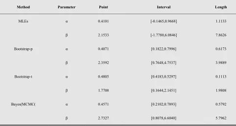
, approximate MLE confidence intervals, Bootstrap confidence intervals and approximate credible intervals based on the MCMC samples, the results are given in Table

2

. The plot of Simulation number of

α

and

β

generated by MCMC method are given in Figures 1 and 2, the plot of histogram of

α

and

β

generated by MCMC method are given in Figures 3 and 4. This was done with

1000

bootstrap sample and

10 000

MCMC sample and discard the first

1000

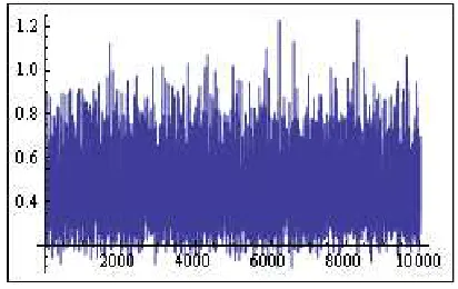
values as `burn-in'

Figure 1. Simulation number of Alfa generated by MCMC.

Figure 2. Simulation number Beta generated by MCMC.

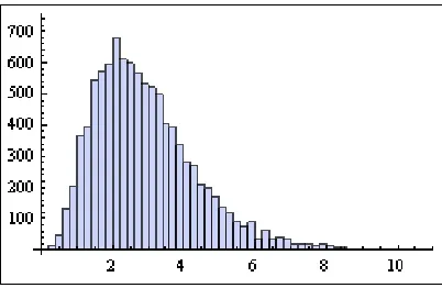
Figure 4. Histogram of Beta generated by MCMC.

6. Simulation Study

In this section we report some numerical experiments performed to evaluate the behavior of the proposed methods, we simulated 1000 progressively first- failure censored samples from a GP(

α β

,

) distribution. The samples were simulated by using the algorithm described in (Balakrishnan and Sandhu, 1995). We used different sample of sizes

( )

n

, different effective sample of sizes

( )

m

, different

k

(

k

=

1, 5),

different hyperparameters

( ,

a

b

,

c

,

d

)

, and different of sampling schemes (i.e., different

R

_i

values).We used two sets of parameter values

α

=

0.2,

2

β

=

and

α

=

0.5,

β

=

1.5

, mainly to compare the MLEs and different Bayes estimators and also to explore their effects on different parameter values. First, we used the noninformative gamma priors for both the parameters, that is, when the hyperparameters are

0

. We call it prior 0:

0.

a

= = = =

b

c

d

Note that as the hyperparameters go to 0, the prior density becomes inversely proportional to its argument and also becomes improper. This density is commonly used as an improper prior for parameters in the range of

0

to infinity, and this prior is not specifically related to the gamma density. For computing Bayes estimators, other than prior 0, we also used informative prior, including prior

1

,

a

=

1,

b

=

1,

c

=

3

and

d

=

2

. In two cases, we used the squared error loss function to compute the Bayes estimates. We also computed the Bayes estimates and

95%

credible intervals based on

10000

MCMC samples and discard the first

1000

values as `burn-in'. We report the average Bayes estimates, mean squared errors (MSEs) , coverage percentages, and average confidence interval lengths. For comparison purposes, we also compute the MLEs and the

95%

confidence intervals based on the observed Fisher information matrix.

Note that Scheme

(0,...,

n

−

m

)

when

k

=

1

is the usual type II censoring scheme for fixed

n

and

m

; that is ,

n

−

m

items are removed at the time of the

m

-th failure. Scheme

(

n

−

m

,..., 0)

is just the opposite of the type II censoring scheme in the sense for fixed

n

and

m

,

n

−

m

items are removed at the time of the first failure. It

is well known that when

k

=

1

for fixed

n

and

m

, the expected experimental time of the type II censoring scheme

(0,...,

n

−

m

)

are less than that for

(

n

−

m

,..., 0)

. In fact, the expected time of any other censoring scheme (for

fixed

m

and

n

) is always between these two extremes; for example, the expected experimental time of Scheme

(0,...,

n

−

m

,..., 0)

lies between Schemes

(

n

−

m

,..., 0)

and

(0,...,

n

−

m

)

. Finally, we used the same

1000

replicates to compute different estimates for

each scheme Tables

3

−

7

report the results based on

MLEs and the Bayes estimators (using both the Gibbs sampling procedure) using noninformative prior and

informative prior on both

α

and

β

.

7. Conclusion

In this paper we consider the Bayes estimation of the unknown parameters of the GP( α β, ) distribution when the data are progressively first-failure censored. We assume the gamma priors on the unknown parameters and provide the Bayes estimators under the assumptions of squared error loss functions. It is observed that the Bayes estimators can not be obtained in explicit forms and they can be obtained using the numerical integration. Because of that we have used MCMC technique to generate posterior sample. We observe the following.

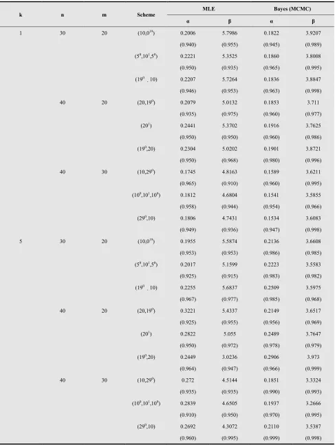
1)From the results obtained in Tables

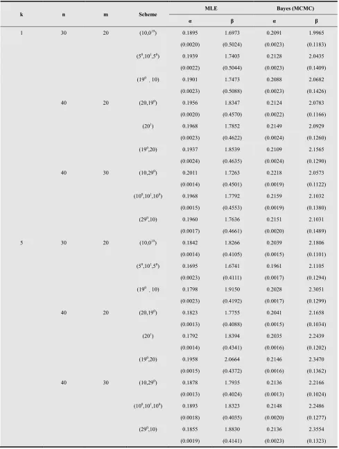
3

and

4

. It can be seen that the performance of the Bayes estimators with respect to the noninformative prior (prior 0) is quite close to that of the MLEs.

2)Tables

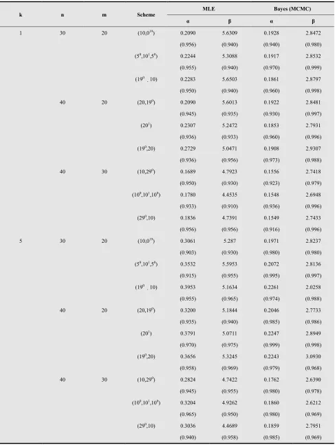
5

and

6

report the results based on informative prior, (prior 1) also in these case the results based on using the Gibbs sampling procedure are quite similar in nature when comparing the Bayes estimators based on informative prior clearly shows that the Bayes estimators based on prior

1

perform better than the MLEs, in terms of both MSEs and lengths of the confidence interval and credible interval.

3)From Tables

3 6

−

, comparing the schemes

(

n

−

m

,..., 0)

and

(0,...,

n

−

m

)

, it is clear that the biases, MSEs, and average confidence interval lengths, credible interval lengths of the MLEs and Bayes estimators for both parameters are greater for the censoring scheme

(0,...,

n

−

m

)

than the censoring scheme

(

n

−

m

,..., 0).

This may not be very surprising, because the expected duration of the experiments is greater for censoring scheme

(

n

−

m

,..., 0)

than for the censoring scheme

(0,...,

n

−

m

)

. Thus the data obtained by the censoring scheme

(

n

−

m

,..., 0)

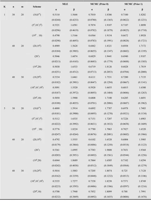
would be expected to provide more information about the unknown parameters than the data obtained by censoring scheme

4)We report the results of MLEs and Bayes estimators based on the Gibbs sampling procedure. For

α

=

0.5

and

β

=

1.5

, the average values of the MLEs, Bayes estimates based on (prior 0) and (prior 1) and corresponding MSEs, are reported in Table

7

. The performance of the Bayes estimators based on prior

0

is very similar of the corresponding Bayes estimators based on prior

1

. From Table

7

, it is clear that the Bayes estimators based on noninformative prior and informative prior perform much better than the MLEs in terms of biases, MSEs.

Table 1. Simulated data from Generalized Pareto with (α,β)=(0.5,2).

14.576 4.7854 1.3924 540.16 1.3164 1.1806 27.308 0.2579

1.3966 37.737 0.2881 183.14 3.6364 44.807 21.321 3.3763

42.369 1.3689 467.58 54.511 0.5397 1.1582 0.4332 1.8647

7.1081 0.5800 1.3975 1.6914 4.0923 0.7111 37.294 3.6109

5.0149 5.0759 692.34 6.9195 0.7539 11.714 0.8957 5.4046

2.1283 1.1501 6.3794 157.15 82.834 1.3905 12.284 26.752

8.7481 20.027 4.9856 2.0358 6.5845 1.2483 3.9334 4.7713

20.030 16.654 2.1791 5.1828 29.241 467.58 2.4447 13.872

Table 2. Results obtained by MLE, Bootstrap and MCMC method of α and β.

Method Parameter Point Interval Length

MLEs α 0.4101 [-0.1465,0.9668] 1.1133

β 2.1533 [-1.7780,6.0846] 7.8626

Bootstrap-p α 0.4071 [0.1822,0.7996] 0.6173

β 2.3592 [0.7648,4.7537] 3.9889

Bootstrap-t α 0.4805 [0.4183,0.5297] 0.1113

β 1.7708 [0.1644,2.1451] 1.9808

Bayes(MCMC( α 0.4571 [0.2102,0.7893] 0.5792

Table 3. Average values of the different estimators and the corresponding MSEs when α=0.2 and β=2 with prior 0.

k n m Scheme

MLE Bayes (MCMC)

α β α β

1 30 20 (10,019) 0.1895 1.6973 0.2091 1.9965

(0.0020) (0.5024) (0.0023) (0.1183)

(50_,101_,50_{) 0.1939 1.7403 0.2128 2.0435}

(0.0022) (0.5044) (0.0023) (0.1409)

(190 _10)

 0.1901 1.7473 0.2088 2.0682

(0.0023) (0.5088) (0.0023) (0.1426)

40 20 (20,190_{) 0.1956 1.8347 0.2124 2.0783}

(0.0020) (0.4570) (0.0022) (0.1166)

(201_{) 0.1968 1.7852 0.2149 2.0929}

(0.0023) (0.4622) (0.0024) (0.1260)

(190,20) 0.1937 1.8539 0.2109 2.1565

(0.0024) (0.4635) (0.0024) (0.1290)

40 30 (10,290_{) 0.2011 1.7263 0.2218 2.0573}

(0.0014) (0.4501) (0.0019) (0.1122)

(100_,101_,100_{) 0.1968 1.7792 0.2159 2.1032}

(0.0015) (0.4553) (0.0019) (0.1380)

(290_{,10) 0.1960 1.7636 0.2151 2.1031}

(0.0017) (0.4661) (0.0020) (0.1489)

5 30 20 (10,019_{) 0.1842 1.8266 0.2039 2.1806}

(0.0014) (0.4105) (0.0015) (0.1101)

(50,101,50) 0.1695 1.6741 0.1961 2.1105

(0.0023) (0.4111) (0.0017) (0.1294)

(190 _10)

 0.1798 1.9150 0.2028 2.3051

(0.0023) (0.4192) (0.0017) (0.1299)

40 20 (20,190_{) 0.1823 1.7755 0.2041 2.1658}

(0.0013) (0.4088) (0.0015) (0.1034)

(201_{) 0.1792 1.8394 0.2035 2.2439}

(0.0014) (0.4341) (0.0016) (0.1202)

(190_{,20) 0.1958 2.0664 0.2146 2.3470}

(0.0015) (0.4372) (0.0016) (0.1362)

40 30 (10,290) 0.1878 1.7935 0.2136 2.2166

(0.0013) (0.4024) (0.0013) (0.1024)

(100_,101_,100_{) 0.1893 1.8323 0.2148 2.2486}

(0.0018) (0.4035) (0.0020) (0.1277)

(290_{,10) 0.1855 1.8830 0.2136 2.3554}

(0.0019) (0.4141) (0.0023) (0.1323)

Table 4. Average confidence interval, credible interval lengths and the coverage percentages when α=0.2 and β=2 with prior 0.

k n m Scheme

MLE Bayes (MCMC)

α β α β

1 30 20 (10,019_{) 0.2006 5.7986 0.1822 3.9207}

(0.940) (0.955) (0.945) (0.989)

(50_,101_,50_{) 0.2221 5.3525 0.1860 3.8008}

(0.950) (0.935) (0.965) (0.995)

(190 _10)

 0.2207 5.7264 0.1836 3.8847

(0.946) (0.953) (0.963) (0.998)

40 20 (20,190_{) 0.2079 5.0132 0.1853 3.711}

(0.935) (0.975) (0.960) (0.977)

(201_{) 0.2441 5.3702 0.1916 3.7625}

(0.950) (0.950) (0.960) (0.986)

(190_{,20) 0.2304 5.0202 0.1901 3.8721}

(0.950) (0.968) (0.980) (0.996)

40 30 (10,290_{) 0.1745 4.8163 0.1589 3.6211}

(0.965) (0.910) (0.960) (0.995)

(100_,101_,100_{) 0.1812 4.6804 0.1541 3.5855}

(0.958) (0.944) (0.954) (0.966)

(290_{,10) 0.1806 4.7431 0.1534 3.6083}

(0.949) (0.936) (0.947) (0.998)

5 30 20 (10,019_{) 0.1955 5.5874 0.2136 3.6608}

(0.953) (0.953) (0.986) (0.985)

(50_,101_,50_{) 0.2017 5.1599 0.2223 3.5583}

(0.925) (0.915) (0.983) (0.982)

(190 _10)

 0.2255 5.6837 0.2509 3.5975

(0.967) (0.977) (0.985) (0.968)

40 20 (20,190_{) 0.3221 5.4337 0.2149 3.6517}

(0.925) (0.955) (0.956) (0.969)

(201_{) 0.2822 5.055 0.2489 3.7647}

(0.950) (0.972) (0.978) (0.979)

(190_{,20) 0.2449 3.0236 0.2906 3.973}

(0.964) (0.947) (0.966) (0.999)

40 30 (10,290_{) 0.272 4.5144 0.1851 3.3324}

(0.935) (0.935) (0.990) (0.993)

(100_,101_,100_{) 0.2839 4.6505 0.1937 3.2666}

(0.910) (0.950) (0.970) (0.995)

(290_{,10) 0.2692 4.3072 0.2110 3.5387}

(0.960) (0.995) (0.999) (0.998)

Table 5. Average values of the different estimators and the corresponding MSEswhen α=0.2 and β=2 with prior 1.

k n m Scheme

MLE Bayes (MCMC)

α β α β

1 30 20 (10,019_{) 0.1967 1.6867 0.2261 1.7885}

(0.0020) (0.5045) (0.0020) (0.0891)

(50_,101_,50_{) 0.1952 1.7072 0.2237 1.8342}

(0.0028) (0.5065) (0.0024) (0.0916)

(190 _10)

 0.1903 1.7339 0.2168 1.8397

(0.0029) (0.5381) (0.0028) (0.0959)

40 20 (20,190_{) 0.1964 1.7165 0.2253 1.8074}

(0.0020) (0.5025) (0.0020) (0.0805)

(201_{) 0.1892 1.7508 0.2151 1.8572}

(0.0021) (0.5110) (0.0022) (0.0823)

(190_{,20) 0.1930 1.8173 0.2173 1.9135}

(0.0024) (0.5131) (0.0023) (0.0828)

40 30 (10,290_{) 0.1953 1.7073 0.2218 1.8229}

(0.0016) (0.5020) (0.0020) (0.0795)

(100_,101_,100_{) 0.1947 1.7045 0.2207 1.8556}

(0.0019) (0.5133) (0.0024) (0.0840)

(290_{,10) 0.1962 1.7664 0.2214 1.8831}

(0.0019) (0.5433) (0.0025) (0.0842)

5 30 20 (10,019_{) 0.1769 1.7423 0.2035 1.9583}

(0.0016) (0.4610) (0.0017) (0.0521)

(50_,101_,50_{) 0.1765 1.7951 0.2023 1.9951}

(0.0018) (0.4643) (0.0019) (0.0541)

(190 _10)

 0.1847 1.9712 0.2055 2.0934

(0.0027) (0.4782) (0.0019) (0.0544)

40 20 (20,190_{) 0.1829 1.7311 0.2114 1.9575}

(0.0015) (0.4362) (0.0016) (0.0467)

(201_{) 0.1777 1.8226 0.2060 2.0529}

(0.0022) (0.4405) (0.0019) (0.0471)

(190_{,20) 0.1964 2.0802 0.2145 2.1446}

(0.0025) (0.4951) (0.0023) (0.0482)

40 30 (10,290_{) 0.1921 1.8746 0.2157 2.0519}

(0.0014) (0.3738) (0.0016) (0.0457)

(100_,101_,100_{) 0.1962 1.9190 0.2196 2.0949}

(0.0026) (0.3766) (0.0019) (0.0557)

(290_{,10) 0.1834 1.9266 0.2056 2.1311}

(0.0027) (0.3881) (0.0020) (0.0571)

Table 6. Average confidence interval, credible interval lengths and the coverage percentages when α=0.2 and β=2 with prior 1.

k n m Scheme

MLE Bayes (MCMC)

α β α β

1 30 20 (10,019_{) 0.2090 5.6309 0.1928 2.8472}

(0.956) (0.940) (0.940) (0.980)

(50_,101_,50_{) 0.2244 5.3088 0.1917 2.8532}

(0.955) (0.940) (0.970) (0.999)

(190 _10)

 0.2283 5.6503 0.1861 2.8797

(0.950) (0.940) (0.960) (0.998)

40 20 (20,190_{) 0.2090 5.6013 0.1922 2.8481}

(0.945) (0.935) (0.930) (0.997)

(201_{) 0.2307 5.2472 0.1853 2.7931}

(0.936) (0.933) (0.960) (0.996)

(190_{,20) 0.2729 5.0471 0.1908 2.9307}

(0.936) (0.956) (0.973) (0.988)

40 30 (10,290_{) 0.1689 4.7923 0.1556 2.7418}

(0.950) (0.930) (0.923) (0.979)

(100_,101_,100_{) 0.1780 4.4535 0.1548 2.6948}

(0.933) (0.910) (0.936) (0.996)

(290_{,10) 0.1836 4.7391 0.1549 2.7433}

(0.956) (0.956) (0.916) (0.996)

5 30 20 (10,019_{) 0.3061 5.287 0.1971 2.8237}

(0.903) (0.930) (0.980) (0.980)

(50_,101_,50_{) 0.3532 5.5953 0.2072 2.8136}

(0.915) (0.955) (0.995) (0.997)

(190 _10)

 0.3953 5.1634 0.2261 2.0258

(0.955) (0.965) (0.974) (0.988)

40 20 (20,190_{) 0.3200 5.1844 0.2046 2.7733}

(0.935) (0.940) (0.985) (0.986)

(201_{) 0.3791 5.0711 0.2247 2.8949}

(0.970) (0.975) (0.999) (0.998)

(190_{,20) 0.3656 5.3245 0.2243 3.0930}

(0.958) (0.969) (0.979) (0.968)

40 30 (10,290_{) 0.2824 4.7422 0.1762 2.6390}

(0.945) (0.955) (0.980) (0.978)

(100_,101_,100_{) 0.3204 4.9262 0.1860 2.6212}

(0.965) (0.950) (0.980) (0.969)

(290_{,10) 0.3036 4.4689 0.1859 2.7951}

(0.940) (0.958) (0.985) (0.969)

Table 7. Average values of the different estimators and the corresponding MSEs when α=0.5 and β=1.5.

K n m Scheme

MLE MCMC (Prior 0) MCMC (Prior 1)

α β α β α β

1 30 20 (10,019_{) 0.5110 1.5646 0.7010 1.8306 0.7100 1.8202}

(0.0244) (0.4233) (0.0780) (0.1365) (0.0822) (0.1231)

(50_,101_,50_{) 0.5321 1.6581 0.7074 1.9107 0.7187 1.8898}

(0.0296) (0.4619) (0.0782) (0.1879) (0.0825) (0.1710)

(190 _10)

 0.4790 1.5166 0.6564 1.9154 0.6672 1.8928

(0.0298) (0.4693) (0.0783) (0.1991) (0.0828) (0.1721)

40 20 (20,190_{) 0.4989 1.5628 0.6842 1.8321 0.6938 1.7172}

(0.0184) (0.3903) (0.0655) (0.1347) (0.0682) (0.1195)

(201_{) 0.5046 1.6074 0.6829 1.9441 0.6940 1.9187}

(0.0213) (0.4165) (0.0683) (0.1779) (0.0688) (0.1303)

(190_{,20) 0.5030 1.6533 0.6719 1.8126 0.6828 1.7819}

(0.0251) (0.4512) (0.0713) (0.2053) (0.0704) (0.2008)

40 30 (10,290_{) 0.5334 1.6461 0.6111 1.7531 0.7200 1.7135}

(0.0182) (0.3901) (0.0647) (0.1294) (0.0667) (0.1141)

(100_,101_,100_{) 0.5091 1.5520 0.5928 1.6655 0.6015 1.6300}

(0.0187) (0.3972) (0.0693) (0.1404) (0.0686) (0.1263)

(290_{,10) 0.5050 1.5900 0.6808 1.7100 0.6285 1.6691}

(0.0188) (0.4035) (0.0701) (0.2086) (0.0687) (0.1962)

5 30 20 (10,019_{) 0.4888 1.5914 0.6892 1.7787 0.6978 1.7403}

(0.0181) (0.3900) (0.0495) (0.1270) (0.0521) (0.1134)

(50_,101_,50_{) 0.5112 1.6535 0.7151 1.7207 0.7226 1.6983}

(0.0222) (0.3992) (0.0631) (0.1832) (0.0658) (0.1609)

(190 _10)

 0.5776 1.8224 0.7780 1.7063 0.7827 1.6520

(0.0247) (0.4264) (0.0676) (0.2001) (0.0682) (0.1966)

40 20 (20,190_{) 0.4792 1.5555 0.6102 1.6528 0.6004 1.5905}

(0.0179) (0.3864) (0.0486) (0.1258) (0.0518) (0.1123)

(201_{) 0.5361 1.6995 0.7583 1.9808 0.7651 1.9368}

(0.0203) (0.3951) (0.0492) (0.1561) (0.0544) (0.1256)

(190_{,20) 0.6044 1.8689 0.7064 1.6505 0.7102 1.6294}

(0.0242) (0.4038) (0.0512) (0.1849) (0.0564) (0.1279)

40 30 (10,290_{) 0.5016 1.5883 0.7205 1.8074 0.725 1.7128}

(0.0162) (0.3359) (0.0448) (0.1232) (0.0513) (0.1106)

(100_,101_,100_{) 0.5335 1.7277 0.7338 1.8238 0.7371 1.8749}

(0.0223) (0.3593) (0.0486) (0.1306) (0.0597) (0.1216)

(290_{,10) 0.5708 1.7948 0.7852 1.8099 0.788 1.7991}

(0.0232) (0.3849) (0.0492) (0.1655) (0.0606) (0.1476)

References

[1] Abd Ellah, A.H. (2003). Bayesian one sample prediction bounds for the Lomax distribution. Indian Journal of Pure and Applied Mathematics, 34, 101-109.

[2] Abd Ellah, A.H. (2006). Comparison of estimates using record statistics from Lomax model : Bayesian and Non Bayesian approaches. Journal of Statistical Research and Training Center, 3, 139-158.

[3] Arnold, B.C. (1983). Pareto distributions. In: Statistical distributions in scientific Work. International Co-operative Publishing House, Burtonsville, MD.

[4] Balakrishnan, N. and Sandhu, R.A. (1995). A simple simulation algorithm for generating progressively type-II censored samples. American Statistics, 49, 229-230. [5] Bryson, M.C. (1974). Heavy-tailed distributions: Properties

and tests. Technometrics, 16(1), 61--68.

[6] Chahkandi, M. and Ganjali, M. (2009). On some lifetime distributions with decreasing failure rate. Computational Statistics and Data Analysis, 53(12), 4433--4440.

[7] Efron, B. (1982). The Bootstrap and other resampling plans, In: CBMS-NSF Regional Conference Seriesin Applied Mathematics, SIAM, Philadelphia, PA.

[8] Habibullah, M. and Ahsanullah, M. (2000). Estimation of parameters of a Pareto distribution by generalized order statistics. Communication in Statistics-Theory and Methods, 29, 1597-1609.

[9] Hall, P. (1988). Theoretical comparison of Bootstrap confidence intervals. Annals of Statistics, 16, 927-953. [10] Johnson, L.G. (1964). Theory and technique of variation

research, Elsevier, Amsterdam.

[11] Jun, C.-H.,Balamurali, S. and Lee, S.-H. (2006) Variables sampling plans for Weibull distributed lifetimes under sudden death testing. IEEE Transaction on Reliability, 55, 53-58.

[12] Lee, W.-C., Wu, L.-W. and Yu, H.-Y. (2007). Statistical inference about the shape parameter of the Bathtub-Shaped distribution under the failure-censored sampling plan. International Journal of Information Management Science, 18, 157-172.

[13] Lomax, K.S. (1954). Business failure: Another example of the analysis of the failure data. JASA, 49, 847-852.

[14] Marshall, A.W. and Olkin, I. (2007). Life distributions structure of nonparametric, semiparametric, and parametric families, Springer, New York, NY.

[15] Metropolis, N., Rosenbluth, A.W., Rosenbluth, M. N., Teller, A. H. and Teller, E. (1953). Equations of state calculations by fast computing machines. Journal of Chemistry and Physics, 21, 1087--1091.

[16] Rezaei, R., Tahmasbi, R. and Mahmoodi, M. (2010). Estimation of P[Y<X] for generalized Pareto distribution. Journal of Statistical Planning and Inference, 140, 480-494. [17] Robert, C.P. and Casella, G. (2004). Monte Carlo statistical

methods, Second edition. Springer: New York.

[18] Soliman, A.A., Abd Ellah, A.H., Abou-Elheggag, N.A. and Modhesh, A.A. (2012a). Estimation from Burr type XII distribution using progressive first-failure censored data. Journal of Statistical Computation and Simulation, iFirst, 1--21.

[19] Soliman, A.A., Abd Ellah, A.H., Abou-Elheggag, N.A. and Abd-Elmougod, G.A. (2012b). Estimation of the parameters of life for Gompertz distribution using progressive first-failure censored data. Computational Statistics and Data Analysis, 56, 2471--2485.

[20] Soliman, A.A., Abd Ellah, A.H., Abou-Elheggag, N.A. and Modhesh, A.A. (2011a). Bayesian inference and prediction of Burr type XII distribution for progressive first-failure censored sampling, Intelligent Information Management, 3, 175-185.

[21] Soliman, A.A., Abd Ellah, A.H., Abou-Elheggag, N.A. and Abd-Elmougod, G.A. ( 2011b). Simulation-based approach to the study of coefficient of variation of Gompertz distribution under progressive first-failure censoring. Indian Journal of Pure and Applied Mathematics, 42(5), 335-356. [22] Upadhyay, S.K. and Peshwani, M. (2003). Choice between

Weibull and Lognormal models: A simulation based Bayesian study. Communication in Statistics-Theory and Methods, 32, 381-405.

[23] Wu, J.-W., Hung, W.-L. and Tsai, C.-H. (2003). Estimation of the parameters of the Gompertz distribution under the first-failure-censored sampling plan. Statistics, 37(6), 517-525.

[24] Wu, J.-W. and Yu, H.-Y. (2005). Statistical inference about the shape parameter of the Burr type XII distribution under the failure-censored sampling plan. Applied Mathematics and Computation, 163, 443-482.

[25] Wu, J.-W., Ouyang, T.-R. and Yu, L.-Y. (2001). Limited failure-censored life test for the Weibull distribution, IEEE Transaction on Reliability, 50, 107-111.