Time-to-event analysis to evaluate dormancy status of single-bud cuttings: an example for grapevines

METHODOLOGY

Time-to-event analysis to evaluate

dormancy status of single-bud cuttings:

an example for grapevines

Hector Camargo Alvarez

_{, Melba Salazar‑Gutiérrez}

_{, Diana Zapata}

_{, Markus Keller}

and Gerrit Hoogenboom

Abstract

Background: The reduced growth of plants during the winter causes a lack in the perceptibility of the phenological events making challenging the study of dormancy. For deciduous crops, dormancy is generally determined by evalu‑ ating budbreak of single‑node cuttings that are exposed to conditions suitable for growth. However, the absence of a statistical basis for analyzing and interpreting the budbreak behavior evaluated as the percent budbreak, the average time to budbreak and the time to reach 50% budbreak, has caused inconsistent and contradictory criteria to identify the dormancy status of different deciduous crops.

Results: In this study, a method was developed to analyze the duration between sampling and budbreak of single‑ node cuttings and to estimate the dormancy status for grapevines (Vitis vinifera L.) based on the time‑to‑event distri‑ bution of the observations. This method estimates the probability curve of budbreak for each sample and classifies each curve into paradormancy, endodormancy, and ecodormancy according to the significance when compared to a sample curve estimated from cuttings collected during paradormancy and referred to as “reference.”

Conclusion: The approach described in this study provided a comparison of the budbreak distribution of cuttings collected during distinct phases with a confidence of 95%. It also allowed the estimation of the date of occurrence of the dormancy stages for two grapevine cultivars ‘Cabernet Sauvignon’ and ‘Chardonnay,’ based on the variability within the sampling season rather than on fixed arbitrary criteria. This approach can also be used to analyze budbreak data of single‑node cuttings from other common deciduous crops.

Keywords: Survival analysis, Phenology, Endodormancy, Paradormancy, Ecodormancy, Budbreak, Chardonnay, Cabernet Sauvignon, Vitis vinifera L.

© The Author(s) 2018. This article is distributed under the terms of the Creative Commons Attribution 4.0 International License (http://creat iveco mmons .org/licen ses/by/4.0/), which permits unrestricted use, distribution, and reproduction in any medium, provided you give appropriate credit to the original author(s) and the source, provide a link to the Creative Commons license, and indicate if changes were made. The Creative Commons Public Domain Dedication waiver (http://creat iveco mmons .org/ publi cdoma in/zero/1.0/) applies to the data made available in this article, unless otherwise stated.

Background

Plant dormancy can be classified into three differ-ent phases: paradormancy, endodormancy, and eco-dormancy. Paradormancy refers to the period of bud dormancy induced by a structure other than the buds, primarily related to the phenomenon of apical domi-nance [1, 2]. During the subsequent period; endodor-mancy, development and growth are controlled by the perception within the bud of an environmental signal.

Structures in this state are incapable of growth and devel-opment even if the external physiological signals are removed and returned to growth-promoting conditions [2, 3]. Endodormant buds avoid budbreak in response to a transient warming time during late autumn and the subsequent potential damage due to frost. Also, endo-dormancy is part of the process by which buds adapt to winter conditions and it is a prerequisite for the subse-quent acquisition of full cold hardiness [3, 4]. Therefore, endodormancy starts early in autumn prior to leaf senes-cence [3, 5]. When endodormancy is released, there is a transition to ecodormancy, which is the period preced-ing budbreak when growth is prevented by one or more

Open Access

*Correspondence: [email protected]

1 _{AgWeatherNet Program, Irrigated Agriculture Research and Extension}

environmental factors that are not conducive to growth, but growth is resumed when conditions become favora-ble again [2].

The synchronism between the growing season, dor-mancy phase, and the level of cold acclimation can be used as decision support for frost protection manage-ment and site and cultivar selection [4, 6]. Neverthe-less, it is challenging to research dormancy phenology because of limited activity of the buds and the absence of an on-site method to infer the onset and release of endodormancy [1]. To overcome this limitation, the most commonly used method for estimating the occurrence of endodormancy relies upon the exposure of groups of single-bud cuttings to conditions conducive to growth, known as forcing, with an air temperature around 24 ± 2 °C, a relative humidity between 70 and 90%, and a 15 to 16 h photoperiod [3, 7, 8]. When the elapsed time between sampling and budbreak is long and the percent budbreak is small, buds are endodormant [7]. However, the lack of a statistical basis for analyzing single-node cuttings has resulted in inconsistent criteria and arbi-trary thresholds for determining the endodormancy stage [7, 9]. Buds of single-node cuttings of wine grapes under forcing have been classified as endodormant when required between 30 and 50  days to reach 50% bud-break [10, 11], while in a different study endodormancy was identified as the period when 50% of budbreak was reached after 60  days under forcing [12]. Other studies have reported endodormancy as the period when 50% budbreak was reached after 30 days under forcing based on previous reports for apple, sour cherry and peach [13,

14]. However, an average duration to budbreak between 20 and 40  days was found for peach when buds were endodormant [15]. For cherries, 50% budbreak of single-node cuttings was reached after 21 days during endodor-mancy [16]; and in ‘Sweetheart’ sweet cherry and ‘Gala’ apple, endodormant buds required an average between 20 and 60 days to budbreak [17].

Recent studies have used methods based on time-to-event data or survival analysis to evaluate the depth of dormancy [3, 12, 14, 18]. A parametric approach based on probit models with a log-logistic distribution func-tion was adjusted to budbreak of the single nodes as a function of the time after sampling. The estimated time required to reach 50% budbreak according to this model, a parameter named BR50, was used to describe and

com-pare the depth of dormancy of different sampling dates or groups [3, 14]. Non-parametric methods have also been used, such as the Kaplan–Meier estimator of the time-to-event distribution adjusted to the budbreak of single nodes [12, 18]. The Kaplan–Meier estimator has many advantages for evaluating the distribution of bud-break, such as the ease of calculation, the ability to make

quantitative estimates without assuming a particular functional distribution, and the capability to compare Kaplan–Meier estimators with statistical significance by a log-rank test. The Kaplan–Meier estimator also consid-ers the presence of right-censored observations, defined as the buds that have not broken at the end of the fol-low-up period improving the estimation of the budbreak distribution [19–21]. Therefore, the goal of this study was to apply time-to-event analysis to evaluate the budbreak distribution and to estimate the dormancy stage of single-node cuttings of ‘Cabernet Sauvignon’ and ‘Chardonnay.’

Methods

Forced single‑node cuttings method

Growing shoots and dormant canes of Vitis vinifera L. cvs. ‘Cabernet Sauvignon’ and ‘Chardonnay’ were col-lected starting in August and ending around the first week of December from 2013 to 2016. The samples were obtained from own-rooted grapevines in an experimen-tal vineyard located at the Irrigated Agriculture Research and Extension Center, Washington State University, Prosser, WA (46.3°N; 119.7°W; 355  m above sea level). Meteorological data from the local weather station were provided by the Washington State University Agricul-tural Weather Network Program (AgWeatherNet, http://

weath er.wsu.edu). The vines were planted in 2010 in

north–south-oriented rows and spaced at 2.7 m between rows and 1.8  m within rows. All vines were cordon-trained, spur-pruned, and drip-irrigated according to regional standard practices.

was 215  days for 2013, 224  days for 2014, 238  days for 2015, and 203 days for 2016.

Data analysis

The mean time required to reach budbreak considering only the buds that broke during the time of evaluation and the percent budbreak were calculated as reported in previous studies for each sample and cultivar [7, 8,

10, 11]. In addition, duration to budbreak of each sam-ple and cultivar, including right-censored observations of the buds that did not break within the follow-up period were adjusted to the survival distribution function by the nonparametric Kaplan–Meier method. This method calculates the probability of the absence of budbreak as a function of time after sampling. The absence of budbreak is defined as the probability that budbreak of one single node does not occur. However, for clarity, the analysis was conducted in terms of the probability of budbreak, which is the complement of the probability of the absence of budbreak.

The first sample of each year of the study, collected in August before the onset of endodormancy, was used as a “reference” of the behavior of budbreak when growth was not restricted within the bud and buds were parador-mant. A log-rank test was carried out every year to com-pare the estimated survival distributions of the reference sample against the other collected samples; a significant difference indicates that the buds were endodormant at the sampling date that was compared to the reference.

Kaplan–Meier estimator of the survival function

Let N represent the number of collected buds and t1 < t2 < t3 < ··· < tm denote the distinct times at which the buds break or the last day of the follow-up period when there are right-censored observations. The number of recorded dates of budbreak is represented by m, and j is the index of the observed budbreak times. For each j =1,…, m, m ≤ N because several buds can break at the same tj, in which case the data contain ties. Let Yj be the number of buds at risk (not yet broken) just prior to tj and let bj be the number of buds broken at tj. Then the Kaplan–Meier estimator Ŝ(t) of the survival function is defined as shown in Eq. (1).

This means that the function only changes at values of t at which bj≥1 and the censored data are the buds at risk at the end of the follow-up period [19, 23, 24].

(1) ˆ

S(t)= j:tj<t

1− bj

Yj

Log‑rank test

Let K be the number of samples taken during a year and Sk (t) be the survival function of the kth sample, k= 1,…, K. The hypotheses to be tested are:

where τ is the longest time at which all the groups have at least one subject at risk. Let t1 < t2 < t3 < ··· < tD be the

dis-tinct budbreak times from the pooled sample [24, 25]. Let bi=K

k=1bik be the number of budbreak in the pooled sample at time ti, i = 1,…, D, and let Yi=Kk=1Yik be the number of buds at risk in the combined sample at time ti [23, 24]. The standard log-rank test is based on the statis-tic G, which has the form of a K-vector G=(G1, ...,GK) with:

The variance of Gk is Vkk as defined for Eq. (3) and the covariance between Gk and Gh statistics calculated for the

kth and hth samples is Vkh shown in Eq. (4).

Let V be the estimated variance–covariance matrix formed by the Vkk and Vkh values from Eqs.  (3) and (4). Thus, a K-sample test for HO versus HA has a Chi squared distribution ( χ2 ) and can be calculated as shown in Eq. (5).

When the comparison is performed only between two samples, as in this study when each individual survival dis-tribution was compared against the reference, a two-sided test statistic that compares the kth against the hth samples is used as shown in Eq. (6) and the hypotheses to be tested are:

HO:S1(t)=S2(t)= · · · =SK(t) for allt≤τ, versus

HA:at least one of the Sk(t)’s is different for somet≤τ

(2)

G_k =

D

i=1

b_ik −Y_ikbi Yi

(3)

V_kk =

D

i=1

Yik

Yi

1−Yik Yi

Yi−bi

Yi−1

bi, 1≤k≤K

(4) V_kh=

D i=1 Yik Yi Yih Yi Yi−bi

Yi−1

bi, 1≤k�=h≤K

χ2=(G1,. . .,GK)V−(G1,. . .,GK)′

with K-1 degrees of freedom, and apvalue

(5)

p=Pr(χ2>χ2)

HO:Sk(t)=Sh(t) for allt≤τ, versus

The K-1 samples collected for 1  year were compared against the reference for that year. Then, K-1 two-sam-ple hypotheses were tested simultaneously in a multi-ple comparison test. When multimulti-ple comparisons are performed, the family-wise error rate (FWE), which is the probability of incorrectly rejecting one or more of the K-1 hypotheses simultaneously, is the controlled α rather than the comparison wise error (CWE), which is the probability of incorrectly rejecting a single compari-son or hypothesis. The CWE should be less than or equal to the FWE in order to obtain the exact coverage prob-ability 1-α [24, 26, 27]. Thus, simultaneous p-values for all comparisons were adjusted and scaled according to the variance–covariance matrix using the Dunnett-Hsu adjustment, which increases the χ2 critical value of rejec-tion and consequently decreases the CWE for every sin-gle comparison for an FWE α = 0.05 [23]. The statistical analysis was conducted using the SAS software version 9.4 with PROC LIFETEST (SAS Institute, Cary, NC) [23].

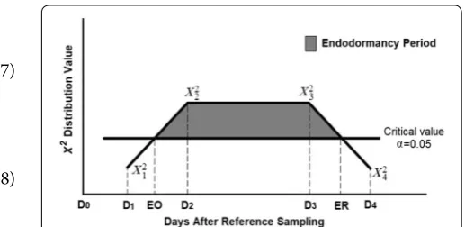
The χ2 values of the comparisons between each sam-ple and the reference were sorted chronologically every year for each cultivar and a straight line was projected between the χ2 values of the first sample with a signifi-cant difference and the preceding sample. The onset of endodormancy was estimated as the date when the line crossed the adjusted critical χ2 value for hypothesis rejec-tion with 95% confidence as defined in Eq. (7). Similarly, the release of endodormancy was estimated as the date of the crossing of the adjusted critical χ2 value with 95% confidence and the straight line obtained between the χ2 values of the last sample with a significant difference and the subsequent sample as defined in Eq. (8). This process was conducted with the Solver tool of Microsoft Office Excel Version 2013.

where EO is the onset of endodormancy, ER is the release of endodormancy, D1 is the date of the sample preceding D2, which is the date of the first sample with significant difference relative to the reference, D3 is the last date (6)

z_kh2 = (Gk−Gh)

2

Vkk+Vhh−2Vkh

p=Pr(χ2>z_kh2) 1 degree of freedom

(7)

EO= (D2−D1)

Cv−χ2₁

χ2₂−χ2₁

+D1

(8)

ER=D4− (D4−D3)

Cv−χ2₄

χ2₃−χ2₄

with significant difference against the reference, and D4 is the date of the subsequent sample. χ2i is the Chi squared value of the comparison between the sample from each Di and the reference, and Cv is the adjusted critical value corresponding to an FWE α = 0.05 (Fig. 1). The compu-tation of adjusted critical values requires arduous calcu-lations [26]. Therefore, in our study computations were made mathematically using either Microsoft Office Excel version 2013 or SAS software version 9.4 with PROC LIFETEST (SAS Institute, Cary, NC) as described in the Additional files 1 and 2.

Results

Average duration to budbreak and percent budbreak

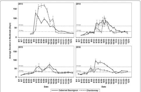
Throughout the 4  years of the evaluation, both grape-vine cultivars showed a period of increase of the aver-age duration to budbreak and reduction of the percent budbreak of the cuttings caused by an internal arrest of bud growth during endodormancy. However, the onset and the end of these events did not coincide during each year. In 2013, for ‘Cabernet Sauvignon’ the average dura-tion to budbreak increased sharply from 23 to 130 days at 4 September and decreased at the end of October, suggesting the end of endodormancy, while the percent budbreak decreased from 100% to 83% only during Sep-tember. In 2014 and 2016, the increase of the average duration to budbreak occurred between the first and sec-ond weeks of September and lasted until the first week of November, while the percent budbreak dropped from mid-August to mid-October. The increase of the average duration to budbreak and reduction of the percent bud-break occurred simultaneously only in 2015 starting the first week of September and ending during the last week of October (Figs. 2, 3).

Fig. 1 Representation of the linear interpolation for estimation of the dates of endodormancy onset (EO) and endodormancy release (ER). The vertical axis represents the X2_{‑value of the comparison between}

For ‘Chardonnay,’ the duration to budbreak in 2013 increased sharply from 18 to 170 days from 4 September until mid-October, when it declined rapidly to 22  days. At the same time, budbreak dropped from 100% to values around 75%. Likewise, in 2016 the duration to budbreak reached values around 100 days, and simultaneously the percent budbreak dropped to 20% from the first week of September to mid-October. During 2014 and 2015, the average duration to budbreak increased more slowly reaching approximately 100 days in 2014 and 60 days in 2015 starting the second week of September until the last week of October. However, in 2014 the percent budbreak decreased from the first week of September until mid-October reaching a minimum of 30%, while in 2015, the decline in budbreak occurred from mid-September until the first week of November, reaching a minimum of 70% (Figs. 2, 3).

Kaplan–Meier estimator and log‑rank test

Although there were marked differences between years in the duration to budbreak, the estimated Kaplan–Meier

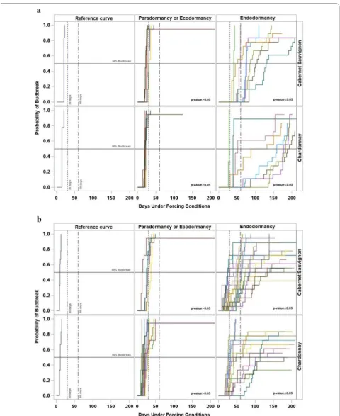
survival functions (curves of probability of budbreak) and the log-rank test showed similar patterns every year with three different periods. The reference curve, esti-mated with paradormant buds, was characterized by a sharp increase in the probability of budbreak during the first 50 days under forcing, with limited to no presence of right-censored observations. The survival curves for the subsequent samples showed a similar response and were not significantly different from the reference curve, suggesting that the buds were still paradormant. The second period was characterized by curves with a slow increase of the probability of budbreak, taking longer than 100  days under forcing for some buds to break. Additionally, during this period there was a higher num-ber of right-censored observations and the samples in this period had probability curves significantly different from the reference curve, suggesting that the buds were endodormant. Finally, during the third period, related to ecodormancy the curves were not significantly different relative to the reference curve, and endodormancy had already occurred.

Each year for both cultivars, 50% percent of budbreak of the reference sample occurred before 30  days under forcing. Similarly, most of the samples that were not sig-nificantly different from the reference required fewer than 30 days under forcing conditions to reach 50% bud-break, with the exception of one sample in 2015 and one sample in 2016 for ‘Chardonnay,’ and three samples in 2013, one sample in 2014 and three samples in 2016 for ‘Cabernet Sauvignon.’ Consequently, most of the sam-ples for both cultivars that showed significant differences against the reference reached 50% budbreak after 30 days under forcing. Except for three samples of each cultivar during 2014, and two samples of ‘Cabernet Sauvignon’ and six samples of ‘Chardonnay’ during 2015 which had numerous right-censored observations (Figs. 4, 5).

In 2013, eight consecutive samples for both cultivars were identified as endodormant starting on 9 Septem-ber and ending on 29 OctoSeptem-ber. Although all the curves with significant differences reached 50% budbreak, in five samples of ‘Chardonnay’ it required more than 100 days (Fig. 4a). In 2014, 21 samples of ‘Cabernet Sauvignon’ between 26 August and 4 November and 16 samples of ‘Chardonnay’ between 2 September and 24 October were

identified as endodormant. The samples collected in 2014 showed numerous curves with right-censored observa-tions; 12 curves in ‘Cabernet Sauvignon’ and 11 curves in ‘Chardonnay’ had a budbreak lower than 80% (Fig. 4b). In 2015, ‘Cabernet Sauvignon’ had eight successive samples between 4 September and 29 October, and ‘Chardonnay’ had seven samples between 11 September and 29 Octo-ber identified as endodormant. The samples collected in 2015 had the lowest amount of right-censored observa-tions; all the curves had percent budbreak equal to or greater than 80% (Fig. 5a). In 2016, eight consecutive sampling dates between 4 September and 14 October for both cultivars were identified as endodormant and none of the curves reached 100% budbreak (Fig. 5b).

Onset of endodormancy and release date estimation

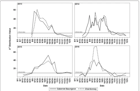
5 September for ‘Cabernet Sauvignon’ and 19 September for ‘Chardonnay”; for 2015, the most profound dormancy occurred on 14 October for both cultivars; and for 2016 it occurred on 16 September for ‘Cabernet Sauvignon’ and between 16 and 22 September for ‘Chardonnay’ (Fig. 6). The estimated onset of endodormancy occurred slightly later each year for ‘Chardonnay’ between 31 August and 6 September, compared to ‘Cabernet Sauvignon,’ which became endodormant between 26 August and 4 Sep-tember. In contrast, the estimated release of endodor-mancy occurred earlier for ‘Chardonnay,’ between 21 October and 3 November, while for ‘Cabernet Sauvignon’ it occurred between 27 October and 5 November. As a result, ‘Chardonnay’ had a shorter endodormancy period than ‘Cabernet Sauvignon’ for each year of the study period (Table 1).

Discussion

During the 4  years of the study, a period characterized by the simultaneous increase of the average duration to budbreak and reduction of percent budbreak of nodes exposed to forcing was quickly identified as endodor-mancy [10, 11]. In contrast, the typical response of

the buds during paradormancy and ecodormancy was characterized by a low average duration to budbreak and simultaneous budbreak close or equal to 100% [12,

13]. However, when the response of the duration to budbreak and percent budbreak was not as clear, gen-erally around the transitions from paradormancy to endodormancy and subsequently to ecodormancy, the determination of the dormancy phase was challenging.

Fig. 6 Chi squared values of the log‑rank comparison between the survival function of each sample against the survival function of the reference sample (non‑dormant first sample of every year) for 2013, 2014, 2015, and 2016. The solid line represents the χ2 _{critical value with an FWE α = 0.05}

Table 1 Estimated dates for  the  onset and  release

of  endodormancy for  ‘Cabernet Sauvignon’

and ‘Chardonnay’ in Prosser, WA

Cultivar Year

2013 2014 2015 2016

Cabernet Sauvignon

Onset 4‑Sep 26‑Aug 4‑Sep 29‑Aug

Release 2‑Nov 5‑Nov 4‑Nov 27‑Oct

Chardonnay

Onset 6‑Sep 2‑Sep 5‑Sep 31‑Aug

An additional limitation was caused by the temporal dif-ferences between both variables as found during 2013, 2014, and 2016 in ‘Cabernet Sauvignon’ and during 2014 and 2015 in ‘Chardonnay,’ when the percent budbreak tended to decrease 1 or 2 weeks earlier than the increase of the average duration to budbreak. These temporal dif-ferences can be caused by the early induction of endodor-mancy in a small percentage of buds following the regular cumulative frequency of any phenological stage [28], the genetic variation within the grapevine, variability in bud microclimate, and variability in the distance from the shoot base [29, 30]. These factors affect the percent budbreak earlier than the average duration of budbreak. In addition, the range of duration to budbreak and per-cent budbreak varied every year suggesting that duration to budbreak and percent budbreak cannot be analyzed separately and both variables are complementary to iden-tify endodormancy. For example, during 2014 and 2016 ‘Chardonnay’ had samples with a duration to budbreak that was less than 50  days but a very low percent bud-break, while in 2013 the opposite occurred and the per-cent budbreak was higher than 80% and the duration to budbreak was greater than 100 days.

The annual variation in the range of duration to bud-break and the percent budbud-break also suggests that the estimations of the dormancy phase based on fixed, arbi-trary time thresholds to evaluate 50% of budbreak, such as 30 days under forcing [13] and 60 days under forcing [12], in addition to being inconsistent are very impre-cise, especially if many buds are right-censored. When the average duration to budbreak or the time required by the sample to reach 50% budbreak are compared to these thresholds, the right-censored observations are counted as null, ignoring useful information [8, 9, 17]. On the other hand, the limits at which the duration to budbreak and percent budbreak start to be ‘high’ or ‘low’ are not fixed; they are affected each year by the response of the cultivar to experimental conditions and weather variabil-ity [8]. For instance, differences of only 1 °C in the forc-ing temperature can impact the duration to budbreak of the cuttings [31]. Additionally, temperatures before bud sampling can affect the bud response under forcing con-ditions. Thus, warm air temperatures during shoot devel-opment in V. vinifera stimulate axillary-bud outgrowth, modifying the duration to budbreak of the cuttings [32]. Also, elevated temperatures during dormancy induction can cause slow and shallow dormancy as found in Popu-lus x spp [33].

When the results of this study were analyzed based on time-to-event distributions, the analysis dealt with the synchronicity problem between duration to budbreak and percent budbreak, integrating both variables to esti-mate the curves of probability of budbreak (Figs. 4, 5).

Also, the Kaplan–Meier survival functions and the log-rank test for comparison of survival curves with a 95% of confidence allowed the occurrence estimation of the transitions between paradormancy, endodormancy and ecodormancy. These estimates were based on the vari-ability of the samples under the environmental condi-tions at which plants grew and experimental condicondi-tions at which budbreak was induced, increasing the precision of the estimation related to the fixed threshold meth-ods. The results of the log-rank test were partially con-sistent with the results found when paradormancy and ecodormancy were determined as the period when 50% budbreak occurred before 30 days, mainly for ‘Chardon-nay.’ However, the results were less comparable to deter-mine endodormancy when there was a large number of right-censored observations, such as in 2014 and 2016. This discrepancy caused samples classified as endodor-mant by the log-rank test to be classified as paradorendodor-mant or ecodormant by the fixed threshold method because they showed 50% budbreak before 30 days under forcing, but the sample only reached between 60 and 70% bud-break. Also, in some samples a 50% budbreak was never reached, making the response not interpretable with the fixed threshold method. The results of the log-rank test did not show any relation to the 60-day threshold.

The estimated onset of endodormancy occurred con-sistently between 1 and 6 days earlier each year for ‘Cab-ernet Sauvignon’ compared to ‘Chardonnay’ (Table 1). This difference is caused by the ecotypic variation in sensing the triggering signals for the induction of endo-dormancy, such as photoperiod, temperature, light intensity, and water status [4, 5]. Differences in onset of endodormancy presented in this study diverge with previous results where the onset of endodormancy for ‘Cabernet Sauvignon’ and ‘Chardonnay’ coincided [12]. However, those results were based on monthly and bi-weekly samplings, and thus the difference between culti-vars could have been overlooked.

37]. Additionally, the estimated onset of endodormancy occurred earlier in 2014 and 2016 for both cultivars, with 2014 having the warmest and 2016 having the lowest temperatures during August before the onset of endo-dormancy (Fig. 7). This response could be related to the recently proposed existence of two different pathways of temperature-mediated dormancy induction in woody plants, i.e., a low temperature-induced stress pathway in northern latitude ecotypes, and a warm night tempera-ture-short photoperiod induced pathway that affects all ecotypes [33]. Although this model is still unclear, these pathways may explain the plasticity of dormancy induc-tion development and the adaptainduc-tions of plants to ensure dormancy development under variable autumn tempera-tures, thereby maximizing their growing season [9, 33].

The estimated dates of release of endodormancy occurred between 21 October and 5 November for all years (Table 1); consistent with previous reports for buds of V. vinifera which were already ecodormant dur-ing November and December [6, 12]. The variation in the release of endodormancy between years is mainly related to the chilling requirement, which is the amount of tem-perature below a threshold required to satisfy endodor-mancy and to advance to ecodorendodor-mancy [6, 18]. While the relationship between chilling temperatures and estimated dates of endodormancy release is beyond the scope of this study, it is nonetheless, challenging to deter-mine as the chilling requirement of grapevines is not well described. Grapevines require a low exposure to chill-ing compared to many other deciduous fruit crops like apple or peaches, and chilling has even been considered a facultative rather than an absolute requirement [11,

38]. Trials under controlled conditions have reported dif-ferent thresholds of chilling accumulation. For instance, 11.5  °C for ‘Cabernet Sauvignon’ and ‘Chardonnay’ [6], 6 °C for ‘Cabernet Sauvignon’ [39] and 3 °C for ‘Cabernet Sauvignon’ and − 3  °C for ‘Chardonnay’ were reported as the temperature with the highest efficiency of chill-ing [12]. Furthermore, chilling thresholds estimated from field data have been inconsistent in physiological terms, showing chilling efficiency at temperatures as high as 30  °C for ‘Sangiovese’ and 20  °C for ‘Chardonnay’ [38,

40]. Differences in the release of endodormancy between cultivars were also found; the estimated dates of ‘Char-donnay’ occurred consistently between 1 and 10  days earlier compared to ‘Cabernet Sauvignon.’ Previous reports under controlled conditions also found an ear-lier transition from endodormancy to ecodormancy in ‘Chardonnay’ and a higher requirement of chilling units in ‘Cabernet Sauvignon’ compared to ‘Chardonnay’ using the same threshold of 11.6 °C for both cultivars, causing a more extended endodormancy period in the former cul-tivar [6, 12].

Conclusion

dates were consistent with previous reports and the method could be used to analyze the single-node cuttings results commonly obtained in other deciduous crops.

Additional files

Additional file 1. Mathematical estimation of critical values of χ2 _corre‑

sponding to a FWE α = 005 using Microsoft Office Excel version 2013.

Additional file 2. Computation of critical values of χ2 _{corresponding to a}

FWE α = 0.05 using SAS software version 9.4.

Abbreviations

FWE: family‑wise error; CWE: comparison‑wise error.

Authors’ contribution

HC, MK and GH conceived and designed the study. HC and DZ collected the data. HC and MS interpreted and analyzed the data. HC drafted the manuscript supervised by GH and MS. All authors read and approved the final manuscript.

Author details

1 _{AgWeatherNet Program, Irrigated Agriculture Research and Extension}

Center, Washington State University, Prosser, WA 99350, USA. 2 _Department

of Horticulture, Washington State University, Prosser, WA 99350, USA. 3 _Present

Address: Department of Horticulture, Tree Fruit Research and Extension Center, Washington State University, Wenatchee, WA 98801, USA. 4 _{Present Address:}

Department of Soil and Crop Sciences, Texas A&M University, College Station, TX 77843, USA. 5 _{Present Address: Institute for Sustainable Food Systems,}

University of Florida, Gainesville, FL 32611, USA.

Acknowledgements

This research was funded by the Washington Grape and Wine Research Program. We would like to thank the Washington Wine Foundation and Hogue Ranches, which collaborated on this research project, Rick Hamman and Lynn Mills, who contributed their knowledge and experience, and Dr. Carol Wilker‑ son, who provided editorial comments.

Competing interest

The authors declare that they have no competing interest

Available and requirements

The datasets of the duration to budbreak, the estimated survival curves and the R script are publicly available in Mendeley data with the name ‘Time‑to‑ event analysis to evaluate dormancy status of single‑bud cuttings.’

Consent for publication Not applicable.

Ethics approval and consent to participate Not applicable.

Research with plants

The single node cuttings used in this study were collected from an experi‑ mental vineyard and no species at risk of extinction or wild fauna and flora was related. Besides, institutional, national or international guidelines have complied.

Publisher’s Note

Springer Nature remains neutral with regard to jurisdictional claims in pub‑ lished maps and institutional affiliations.

Received: 10 May 2018 Accepted: 19 October 2018

References

1. Alonso JM, Anson JM, Espiau MT, Socias i Company R. Determination of endodormancy break in almond flower buds by a correlation model using the average temperature of different day intervals and its applica‑ tion to the estimation of chill and heat requirements and blooming date. J Am Soc Hortic Sci. 2005;130:308–18.

2. Lang GG. Dormancy: a new universal terminology. HortScience. 1987;22:817–20.

3. Rubio S, Dantas D, Bressan‑Smith R, Pérez FJ. Relationship between endo‑ dormancy and cold hardiness in grapevine buds. J Plant Growth Regul. 2016;35:266–75.

4. Ferguson JC, Moyer MM, Mills LJ, Hoogenboom G, Keller M. Modeling dormant bud cold hardiness and budbreak in twenty‑three Vitis geno‑ types reveals variation by region of origin. Am J Enol Vitic. 2014;65:59–71. 5. Garris A, Clark L, Owens C, McKay S, Luby J, Mathiason K, et al. Mapping

of photoperiod‑induced growth cessation in the wild grape Vitis riparia. J Am Soc Hortic Sci. 2009;134:261–72.

6. Ferguson JC, Tarara JM, Mills LJ, Grove GG, Keller M. Dynamic thermal time model of cold hardiness for dormant grapevine buds. Ann Bot. 2011;107:389–96.

7. Dennis FG. Problems in standardizing methods for evaluating the chilling requirements for the breaking of dormancy in buds of woody plants. HortScience. 2003;38:347–50.

8. Lavee S, May P. Dormancy of grapevine buds ‑ facts and speculation. Aust J Grape Wine Res. 1997;3:31–46.

9. Campoy JA, Ruiz D, Egea J. Dormancy in temperate fruit trees in a global warming context: a review. Sci Hortic. 2011;130:357–72.

10. Dokoozlian NK, Williams LE, Neja RA. Chilling exposure and hydrogen cyanamide interact in breaking dormancy of grape buds. HortScience. 1995;30:1244–7.

11. Dokoozlian N. Chilling temperature and duration interact on the bud‑ break of “Perlette” grapevine cuttings. HortScience. 1999;34:1–3. 12. Cragin J, Serpe M, Keller M, Shellie K. Dormancy and cold hardiness transi‑

tions in winegrape cultivars chardonnay and cabernet sauvignon. Am J Enol Vitic. 2017;68:195–202.

13. Ben Mohamed H, Vadel AM, Geuns JMC, Khemira H. Biochemical changes in dormant grapevine shoot tissues in response to chilling: possible role in dormancy release. Sci Hortic. 2010;124:440–7.

14. Pérez FJ, Rubio S, Ormeño‑Núñez J. Is erratic bud‑break in grapevines grown in warm winter areas related to disturbances in mitochon‑ drial respiratory capacity and oxidative metabolism? Funct Plant Biol. 2007;34:624–32.

15. Gariglio N, González Rossia DE, Mendow M, Reig C, Agusti M. Effect of artificial chilling on the depth of endodormancy and vegetative and flower budbreak of peach and nectarine cultivars using excised shoots. Sci Hortic. 2006;108:371–7.

16. Kuden A, Imrak B, Bayazit S, Comlekcioglu S, Kuden A. Chilling require‑ ments of cherries grown under subtropical conditions of Adana. Middle East J Sci Res. 2012;12:1497–501.

17. Guak S, Neilsen D. Chill unit models for predicting dormancy comple‑ tion of floral buds in apple and sweet cherry. Hortic Environ Biotechnol. 2013;54:29–36.

18. Londo JP, Johnson LM. Variation in the chilling requirement and budburst rate of wild Vitis species. Environ Exp Bot. 2014;106:138–47.

19. McNair JN, Sunkara A, Frobish D. How to analyse seed germination data using statistical time‑to‑event analysis: non‑parametric and semi‑para‑ metric methods. Seed Sci Res. 2012;22:77–95.

20. Altman DG, Bland JM. Time to event (survival) data. BMJ. 1998;317:468–9. 21. Borovkova S. Analysis of survival data. Nieuw Archief voor Wiskunde.

2002;5(3):302–7.

22. Coombe B. Grapevine growth stages—the modified E‑L system. Aus J Grape Wine Res. 1995;1:104–10.

23. SAS Institute Inc. SAS/STAT 13.1 User Guide. SAS/STAT 13.1 User Guide. Cary, NC: SAS Institute Inc.; 2013.

24. Klein J, Moeschberger M. Survival analysis techniques for censored and truncated data. In: Dietz K, Gail M, Krickeberg K, Tsiatis A, Samet J, editors. ACM SIGPLAN notices. 2nd ed. New York: Springer; 2003.

•fast, convenient online submission •

thorough peer review by experienced researchers in your field • rapid publication on acceptance

• support for research data, including large and complex data types •

gold Open Access which fosters wider collaboration and increased citations maximum visibility for your research: over 100M website views per year •

At BMC, research is always in progress.

Learn more biomedcentral.com/submissions

Ready to submit your research? Choose BMC and benefit from:

26. Orelien JG. Computation of p values for multiple comparisons with a control in the SAS System. In: 8th annual conference of SouthEast SAS users group conference. Charlotte, NC; 2000.

27. Hsu JC. The factor analytic approach to simultaneous inference in the general linear model. Journal of Computational and Graphical Statistics. 1992;1:151–68.

28. Schwartz MD. Phenology: an integrative environmental science. New York: Springer; 2013.

29. Chuine I, Bonhomme M, Legave JM, Garcia de Cortazar‑Atauri I, Charrier G, Lacointe A, et al. Can phenological models predict tree phenology accurately in the future? The unrevealed hurdle of endodormancy break. Glob Change Biol. 2016;22:3444–60.

30. May P. From bud to berry, with special reference to inflorescence and bunch morphology in Vitis vinifera L. Aust J Grape Wine Res. 2000;6:82–98. 31. Antcliff A, May P. Dormancy and bud burst in Sultana vines. Vitis.

1961;3:1–14.

32. Keller M, Tarara JM. Warm spring temperatures induce persistent season‑long changes in shoot development in grapevines. Ann Bot. 2010;106:131–41.

33. Tanino KK, Kalcsits L, Silim S, Kendall E, Gray GR. Temperature‑driven plasticity in growth cessation and dormancy development in decidu‑ ous woody plants: a working hypothesis suggesting how molecular and cellular function is affected by temperature during dormancy induction. Plant Mol Biol. 2010;73:49–65.

34. Grant TNL, Gargrave J, Dami IE. Morphological, physiological, and bio‑ chemical changes in Vitis genotypes in response to photoperiod regimes. Am J Enol Vitic. 2013;64:466–75.

35. Wareing PF. Photoperiodism in woody plants. Annu Rev Plant Physiol. 1956;7:191–214.

36. Fennell A. Freezing tolerance and injury in grapevines. J Crop Improv. 2004;10:201–35.

37. Heide OM. Temperature rather than photoperiod controls growth cessa‑ tion and dormancy in Sorbus species. J Exp Bot. 2011;62:5397–404. 38. Fila G, Di Lena B, Gardiman M, Storchi P, Tomasi D, Silvestroni O, et al. Cali‑

bration and validation of grapevine budburst models using growth‑room experiments as data source. Agric For Meteorol [Internet]. 2012;160:69– 79. https ://doi.org/10.1016/j.agrfo rmet.2012.03.003.

39. Vasconcelos R, Pozzobom A, Pires E, Monteiro M, Marques M, Paioli EJ, et al. Effects of chilling and garlic extract on bud dormancy release in cabernet sauvignon grapevine cuttings. Am J Enol Vitic [Internet]. 2007;58:402–4 [cited 2017 Mar 21].