An Apriori-based Approach for First-Order Temporal Pattern

An Apriori-based Approach for First-Order Temporal Pattern

Mining

Sandra de Amo1_{,Daniel A. Furtado}2_{, Arnaud Giacometti}2_{, Dominique Laurent}3 1 _{Universidade Federal de Uberlˆandia, Computer Science Department - Uberlˆandia - Brazil}

[email protected], [email protected] 2 _{LI-Universit´e de Tours, UFR de Sciences - Blois - France}

[email protected] 3

ETIS-CNRS-ENSEA-Universit´e de Cergy Pontoise - Cergy Pontoise - France [email protected]

Abstract. Previous studies on mining sequential patterns have focused on temporal patterns specified by some form of propositionaltemporal logic. However, there are some interesting sequential patterns whose specification needs a more expressive formalism, thefirst-ordertemporal logic. In this article, we focus on the problem of miningmulti-sequential patterns which are first-order temporal patterns (not expressible in propositional temporal logic). We propose two Apriori-based algorithms to perform this mining task. The first one, the PM (Projection Miner) Algorithm adapts the key idea of the classical GSP algorithm for propositional sequential pattern mining by projecting the first-order pattern in two propositional components during the candidate generation and pruning phases. The second algorithm, the SM (Simultaneous Miner) Algorithm, executes the candidate generation and pruning phases without decomposing the pattern, that is, the mining process, in some extent, does not reduce itself to its propositional counterpart. Our extensive experiments shows that SM scales up far better than PM.

Categories and Subject Descriptors: Information Systems [Miscellaneous]: Databases

Keywords: Temporal Data Mining, Sequence Mining, Sequential Patterns, Temporal Data Mining, Frequent Patterns, Knowledge Discovery

1. INTRODUCTION

The problem of discovering sequential patterns in temporal data has been extensively studied in several recent papers ([Agrawal and Srikant 1995; 1996; Zaki 2001; Han et al. 2000; Pinto et al. 2001]) and its importance is fully justified by the great number of potential application domains where mining sequential patterns appears as a crucial issue, such as financial market (evolution of stock market shares quotations), retailing (evolution of clients purchases), medicine (evolution of patients symptoms), local weather forecast, telecommunication (sequences of alarms output by network switches), etc. Different kinds of temporal patterns have been proposed ([Mannila et al. 1997; Bettini et al. 1996; Das et al. 1998; Lu et al. 2000]), as well as general formalisms and algorithms for expressing and mining them have been developed ([Joshi et al. 1999; Padmanabhan and Tuzhilin 1996; Berger and Tuzhilin 1999]). Most of these patterns are specified by formalisms which are, in some extent, reducible to Propositional Temporal Logic. For instance, let us consider the (propositional) sequential pattern of formhi1, i2, . . . , ini(where ij, j ∈ {1, ..., n}, are sets of items) that have been extensively studied in

the literature in the past years ([Agrawal and Srikant 1995; 1996; Zaki 2001; Han et al. 2000]). This

pattern is consideredfrequent if at least α% of clients (αis the minimum support specified by the

user) buy the items ofij sequentially, i.e., the items of i1 are bought at timet1, the items ofi2 are bought at timet2, and so on, witht1< t2< ... < tn. Denoting bypjk (k= 1, ..., nj) the propositional

variables representing the items inij, this pattern can be expressed in Propositional Temporal Logic

by the formulai1∧ ♦(i2∧ ♦(i3∧(. . .∧ ♦in)...)), where ij is the formula (pj₁∧pj₂∧. . . pjnj) and ♦is

the temporal operatorsometimes in the future.

Recent research in Inductive Logic Programming (ILP) ([Masson and Jacquenet 2002; Lee and Raedt 2002]) proposed temporal formalisms which are more expressive than the ones used so far for modeling sequential patterns. Indeed, usual formalisms based on propositional temporal logic are not expressive enough to specify many frequent patterns, like Unix-users logs, for instance [Jacobs and Blockeel 2001]. Undoubtedly, the need for more expressive formalisms to specify temporal patterns arise naturally, as well as methods for mining them in a large amount of data.

In this article, we propose a new kind of temporal pattern, calledmulti-sequential pattern (ormsp), which is not expressible in Propositional Temporal Logic. Such patterns appear in several application domains like financial market, retailing, and roughly speaking aim at representing the behavior of individuals related to each other by some criteria, throughout time. The following situations are

examples of multi-sequential patterns: (a) the quotations of sharesx, ybelonging to the same holding

company frequently present the following behavior: an increase of n points of x is followed by an

increase of m points of y and an ulterior decrease of k points of y; (b) clients x and y working in

the same place usually present the following purchasing behavior: when client x buys a computer

M, some time later his(her) colleaguey buys the same computerM, then clientxbuys a printerP,

which is followed by y purchasing the same printer P. Contrarily to the (propositional) sequential

patterns studied so far ([Agrawal and Srikant 1995; 1996; Zaki 2001; Han et al. 2000]), multi-sequential patterns are not expressible in Propositional Temporal Logic and need the expressive power of First-Order Temporal Logic for their specification. For instance, the pattern expressing the behaviour of stock market shares belonging to a same holding company can be specified by the following first-order temporal formula (∃x1∃x2)(group(x1, x2)∧up(x1, n)∧ ♦(up(x2, m)∧ ♦down(x1, k))).

Besides proposing a new kind of sequential pattern that needs a more expressive formalism than

the usual Propositional Temporal Logic, we also propose two algorithms for mining them: Projection

Miner (PM) andSimultaneous Miner(SM). The first one is based on a technique that decomposes the multi-sequential patterns in two propositional sequential patterns during the candidate generation and pruning phases. So, the mining process can be achieved by adapting the classical GSP algorithm for (propositional) sequential pattern mining. In the second algorithm, the mining technique is carried out without decomposing the pattern. We also present an extensive set of experimental results which allow us to conclude that SM executes three times faster than PM. In our opinion, the main contribution of

this article is to show that a classical Apriori-like technique based on candidate generation, pruning

and validation can be used to mine first-order temporal patterns, and that apurefirst-order technique (SM) produces better results than a technique (PM) adapted from classical methods for propositional sequential pattern mining. It is important to emphasize that both algorithms are not based on temporal logic concepts. Actually, temporal logic is used just as a formalism for expressing the temporal patterns.

The article is organized as follows. In Section 2, we formalize the multi-sequential discovery problem,

using a moreoperational formalism to represent them, i.e., a bi-dimensional array representation. In

Section 3, we present the first algorithm PM. In Section 4, we present the algorithm SM, where

the mining process does not involve decomposing the array in twolinear sequential components. In

Section 5 we analyse the experimental results carried out over synthetic datasets. Finally, in Section 6 we discuss ongoing and further research.

2. PROBLEM FORMALIZATION

the elements ofC clients1_{. Items are denoted by a, b, c, ...and client ids byc}

1, c2, c3, .... For the sake

of simplifying the presentation, we just consider sequence patterns whose elements areitems instead

ofitemsets. Indeed, since the main goal of this article is to investigate the problem of mining sets of sequences, we believe that considering sequences of itemsets could add unnecessary difficulty to the problem we are interested in.

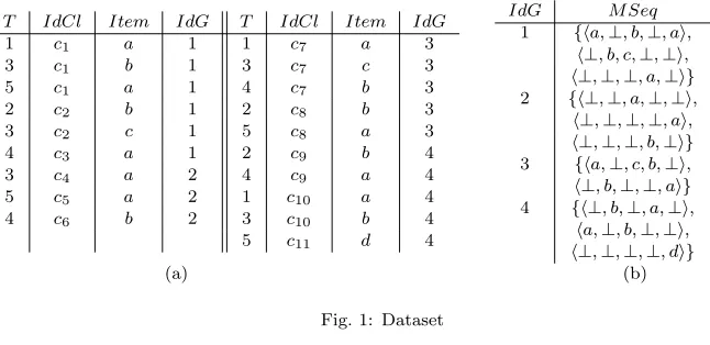
Let us consider a database schemaD={T r(T, IdCl, Item, IdG)}, and a datasetDas an instance

ofD. Here,T is the time attribute whose domain (denoted dom(T)) isN_{. AttributesIdCl,Itemand}

IdGstand for client identifiers, items and group identifiers respectively. Their domain are C, I and

N_{respectively. The table shown in Figure 1(a) is a dataset.}

T IdCl Item IdG T IdCl Item IdG

1 c1 a 1 1 c7 a 3

3 c1 b 1 3 c7 c 3

5 c1 a 1 4 c7 b 3

2 c2 b 1 2 c8 b 3

3 c2 c 1 5 c8 a 3

4 c3 a 1 2 c9 b 4

3 c4 a 2 4 c9 a 4

5 c5 a 2 1 c10 a 4

4 c6 b 2 3 c10 b 4

5 c11 d 4

IdG M Seq

1 {ha,⊥, b,⊥, ai, h⊥, b, c,⊥,⊥i, h⊥,⊥,⊥, a,⊥i}

2 {h⊥,⊥, a,⊥,⊥i,

h⊥,⊥,⊥,⊥, ai, h⊥,⊥,⊥, b,⊥i}

3 {ha,⊥, c, b,⊥i, h⊥, b,⊥,⊥, ai}

4 {h⊥, b,⊥, a,⊥i,

ha,⊥, b,⊥,⊥i, h⊥,⊥,⊥,⊥, di}

(a) (b)

Fig. 1: Dataset

The notions ofsequenceandmulti-sequencein our approach are defined as follows.

Definition2.1 A sequence is a list s = hi1, . . . , iki, where every element ij is in I ∪ {⊥}. The

symbol⊥stands for “don’t care”, andk is called thelengthofs, denoted by|s|.

A multi-sequence is a finite set σ = {s1_{, . . . , s}n_{}, where everys}i _{is a sequence, and for all i, j ∈}

{1, . . . , n} we have | si _{| = | s}j _{| = k. k is called the length of σ and is denoted l(σ). The j-th}

component of sequencesi _{is denoteds}i j.

We notice that each sequencesi ofσis associated to a client of the group.

A dataset can be easily transformed into a table of pairs (g, m) where g is a group identifier and

ma multi-sequence. Figure 1 (b) illustrates this transformation for the datasetD of Figure 1(a). If

(g, m) is in the transformed dataset then we denotembyS(g).

Definition2.2 A multi-sequential pattern (or msp for short) is a multi-sequence satisfying the fol-lowing conditions:

(1) For everyj in{1, . . . , k}there existsiin {1, . . . , n}such thatsi

j is in I and for alll6=i,s l j =⊥.

(2) For everyi in{1, . . . , n} there existsj in {1, . . . , k}such thatsij 6=⊥.

The cardinality ofσis called therank ofσand is denoted by r(σ).

1_{Depending on the application,itemscan be interpreted as articles in a supermarket, stock marketup(n)anddown(p),}

Multi-sequences can be represented by a bi-dimensional array where rows are related to clients and

columns (bottom-up ordered) are related to time. Formsps2_{, the conditions (1) and (2) above are}

interpreted in the array representation as follows: (1) enforces that for each row, there exists a unique position containing an item and all the other positions contain the element⊥. Intuitively, this condition means that at each time we focus only on one client purchases. (2) means that for each column there exists at least one position containing an item. The following example illustrates this definition.

Example2.1 Let us consider the five arrays depicted below. The array (a) represents the

multi-sequential pattern σ ={ha,⊥i,h⊥, ci} whose length and rank are both 2. It is clear that the two

conditions above are satisfied. The same happens for the array (e), whose length is 4 and rank is 3. Arrays (b), (c) and (d) do not represent multi-sequential patterns. Indeed, in array (b), column 2 contains no items (condition (2) is not satisfied); in array (c), row 1 contains two items (condition (1) is not satisfied); and in array (d), row 2 contains no items (condition (1) is not satisfied).

„

⊥ c

a ⊥

«

0

@

c ⊥

b ⊥

a ⊥

1

A

„

⊥ ⊥ a

b c ⊥

«

0

@

b ⊥ a

1

A

0

B B @

⊥ ⊥ d

⊥ c ⊥

b ⊥ ⊥

a ⊥ ⊥

1

C C A

(a) (b) (c) (d) (e)

It is clear that ifσis anmsp, thenr(σ)≤l(σ). We denote by Σn

k the set ofmsps of ranknand length

k.

In order to compare multi-sequences, we define an order relation between elementsx, y ∈ I ∪ {⊥}

as follows: xy ifx=y or x=⊥.

Definition2.3 Letσ={s1, ..., sm}andτ ={t1, . . . , tn}be two multi-sequences. We say thatσis a sub-multi-sequenceof τ (orσisincluded in τ), denoted byσ⊆τ, if there existj1, ..., jm in{1, ..., n}

andi1, ..., ik such that:

—jp6=jq forp6=q

—k=l(σ) andi1< ... < ik

—for allp∈ {1, ..., m}andq∈ {1, ..., k},spq t jp iq.

If we consider the array representations ofσandτ,σ⊆τmeans thatσcan be obtained by considering columnsj1, ..., jmand rowsi1< ... < ik in τ. So, ifσ⊆τ thenl(σ)≤l(τ) andr(σ)≤r(τ).

Example2.2 Let us consider the multi-sequencesσandτ depicted below.

σ=

„

⊥ c

a ⊥

«

τ=

0

@

f e c

⊥ b ⊥

a d d

1

A

It is clear thatσ⊆τ because if we consider rows 1 and 3 and columns 1 and 3 inτ, we obtain an

mspθ (withl(θ) =r(θ) = 2) such thatσi

j θij for eachi= 1,2 andj= 1,2.

Moreover, it should be noticed thatσ is anmsp, whereasτ is not. We emphasize in this respect

that the inclusion relation⊆is defined over multi-sequences in general, and not only overmsps.

Frequentmsps are defined as follows.

Definition2.4 LetDbe a dataset in its transformed version and (g, S(g))∈D. We say thatg sup-portsanmspσifσ⊆S(g). Thesupport of anmspσis defined by: sup(σ) =|{g|g∈ΠIdGDandg supportsσ}|

|D| .

Anmsp σis said to befrequent if sup(σ)≥α, whereαis a given minimum support threshold.

For instance, if we consider the datasetD of Figure 1, themsp of Example 2.1(a) is supported only

by group 1. So, its support is 0.25, and forα= 0.2, thismsp is frequent. As shown in the following

proposition,msp frequency is an anti-monotonic property.

Proposition 2.1 Letσandτ be msps andαa minimum support threshold. Ifσ⊆τ andsup(τ)≥α thensup(σ)≥α.

Problem Formulation. The problem we are interested in can be described as follows: Given a

datasetD and a minimum support thresholdα, find allmsps that are frequent with respect toDand

α.

3. ALGORITHM PM

In this section we describe the algorithmPM (Projection Miner) for miningmsps. The notationsCkn

andLnk are used to denote the set ofcandidate msps andfrequent msps of lengthkand rankn(n≤k)

respectively.

First of all, we show how an msp can be completely characterized by two simple (propositional)

sequences. Letσbe an orderedmsp with l(σ) =kandr(σ) =n. Thecharacteristic function ofσis the functionfσ :{1, ..., k} → {1, ..., n} such that fσ(i) is the number corresponding to the (unique)

column having an element ofI in linei.

Now, we associate toσtwo sequences of lengthk, denoted by Πt(σ) (theitem-sequence ofσ) and

Πs(σ) (theshape-sequence), as follows: Πt(σ) is the projection ofσ over the time axis and Πs(σ) =

hfσ(1), ..., fσ(k)i.

For instance, ifσ is the msp illustrated in case (e) of Example 2.1, then Πt(σ) = ha, b, c, di and

Πs(σ) =h1,1,2,3i.

It is easy to verify that anmspis completely characterized by its shape-sequence and item-sequence.

The numbersk and nare called the length and rank of the shape-sequence Πs(σ) respectively. We

denote by proj(σ) the pair (Πt(σ),Πs(σ)). The inverse function is denoted by ⊠, that is Πt(σ) ⊠

Πs(σ) = σ.

In algorithm PM, the set Ln

k+1 is obtained from L

n k and L

n−1

k . In order to do so, the msps in

Ln

k are projected in two sequence components: a shape-sequence and an item-sequence. At

(sub)-iterationk+ 1 of iterationn, the set of candidate shape-sequences and item-sequences of ranknand

length k+ 1 (denoted CIn

k+1 and CS

n

k+1, respectively) are generated respectively from the sets of

frequent shape-sequencesLSn

k,LS n−1

k and frequent item-sequencesLI

n k,LI

n−1

k , obtained in previous

iterations.

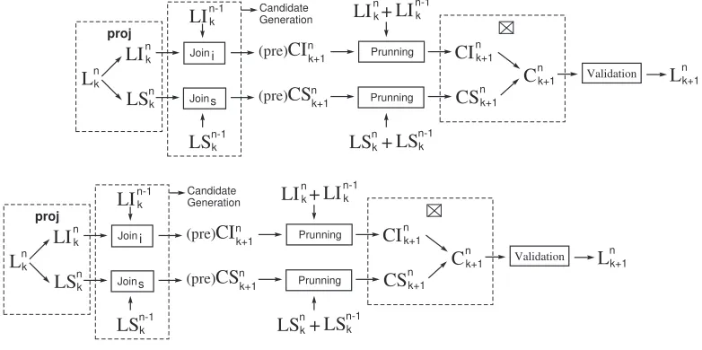
Figure 2 illustrates how the setLn

k+1 is obtained fromL

n k andL

n−1

k .

The algorithm PM is given in Figure 3. At steps3.5and3.9.6, the operator⊠is used to join the

item-sequences and shape-sequences. In this process, each shape-sequence inCSn

k is joined with all

item-sequences ofCIn

k. The resulting set of msps is Ckn (also denoted by CIkn ⊠ CSnk). TheJ oinI

operation joins the item-sequences in LIkn∪LI

n−1

k and returns the set CI

n

k+1 of candidate

L

nk

LI

nk

LS

nk Join

Join

LI

n-1k

LS

n-1k

(pre)

CI

n_k+1

(pre)

CS

n k+1

Prunning

Prunning

LI

n-1k

LS

n-1k

CI

nk+1

CS

nk+1

LI +

nk

LS +

nk

C

nk+1

L

n k+1 Validation i s proj Candidate Generation

L

nk

LI

nk

LS

nk Join

Join

LI

n-1k

LS

n-1k

(pre)

CI

n_k+1

(pre)

CS

n k+1

Prunning

Prunning

LI

n-1k

LS

n-1k

CI

nk+1

CS

nk+1

LI +

nk

LS +

nk

C

nk+1

L

n k+1 Validation i s proj Candidate Generation

Fig. 2: Ln

k+1is obtained fromL

n

k andL

n−1

k

shape-sequences inLSn

k ∪LS n−1

k . The details of these join operations are given in section 3.1 below.

The functionprojcomputes the projections Πi and Πs for allmsps inLnk and returns the setsLIkn

andLSn

k.

3.1 Candidate Generation

TheJ oinIoperation between candidate item-sequences (CI_kn) is computed as in [Agrawal and Srikant

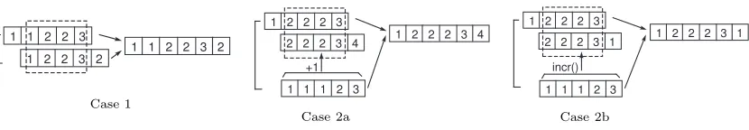
1996]. Concerning the generation of the candidate shape-sequences, there are three possibilities for

computing the result of the J oinS operation. Figure 4 illustrates each of these cases. We explain

below the three cases.

Letσ=hσ1, σ2, ..., σkiandτ=hτ1, τ2, ..., τkibe two shape-sequences of ranknσandnτrespectively.

Let denote byσf irst _{and τ}last _{the sequences obtained by eliminating the first element ofσ and the}

last element ofτ respectively. If σf irst _=τlast _{thenσ andτ are joinable. In this case (Case 1), the}

resulting sequence ishσ1, σ2, ..., σk, τki. Otherwise, we test if τilast+ 1 =σlasti for all i= 1, ..., k. If

this is verified (Case 2a) thenσand τ are joinable and one resulting sequence ishσ1, . . . , σk, τk+ 1i.

We next test (Case 2b) if Inc(τ)last i = σ

last

i for all i = 1, ..., k, where Inc(τ)i = τi+ 1 if τi+ 1 <

max(nσ, nτ) and Inc(τ)i = 1 otherwise. If this is verified then a second resulting sequence is also

obtained, defined ashσ1, . . . , σk, Inc(τ)ki.

The following example illustrates the process of the candidate generation in PM.

Example3.1 Let us suppose thatL2

3 andL13 contain themspsσandτ given below:

σ=   ⊥ c ⊥ b a ⊥ 

andτ =   d c b   γ =     ⊥ d ⊥ c ⊥ b a ⊥    

We joinσandτ in order to obtain the candidate msp γof rank 2 and length 4. We have Πi(σ) =

ha, b, ci ∈LI₃2, Πs(σ) =h1,2,2i ∈LS₃2, Πi(τ) =hb, c, di ∈LI₃1and Πs(τ) =h1,1,1i ∈LS₃1. By joining

Input:α: minimum support, N: number of data multi-sequences, D: dataset

1. k= 0; n= 1;

2. Repeat 2.1k=k+ 1;

2.2L1

k= frequent sequences of rank 1 and lengthk(uses GSP);

2.3 ifL1

k6=∅then {LIk1=L1k; LSk1={h1,1, . . . ,1i} };

UntilL1

k=∅;

3. Repeat

3.1n=n+ 1; k=n;

3.2CIn

n=JoinI(LInn₋−11, LI

n−1

n₋1); (Candidate item-sequences generated fromLI

n−1

n₋1)

3.3CSn

n={h1,2, ..., ni}

3.4 deleteallσ∈CIn

nsuch that∃τ⊆σ,l(τ) =n−1 andτ /∈LI n−1

n₋1 (pruning);

3.5Cn

n=CInn⊠CSnn(build the candidatemsps)

3.6 ForeachgroupginDdo

Increment the count of all candidatemsps inCn

n that are contained inS(g);

3.7Ln

n= candidates inC n

n with count≥αN;

3.8(LIn

n, LSnn) =proj(Lnn); (projects item-sequences and shape-sequences ofLnninto

LIn

n andLSnn);

3.9 Repeat

3.9.1k=k+ 1;

3.9.2CIn

k =JoinI(LI n₋1

k−1∪LI

n k−1, LI

n₋1

k−1 ∪LI

n k−1);

(Candidate item-sequences generated fromLIn−1

k₋1 andLI

n k₋1)

3.9.3 deleteallσ∈CIn

k such that∃τ⊆σ,l(τ) =k−1 andτ /∈LI n₋1

k₋1 ∪LI

n k₋1; (pruning item-sequences)

3.9.4CSn

k =JoinS(LS n₋1

k₋1 ∪LS

n k₋1, LS

n₋1

k₋1 ∪LS

n k₋1); (Candidate shape-sequences generated fromLSn−1

k₋1∪LS

n k₋1)

3.9.5 deleteallσ∈CSn

k such that∃τ⊆σandτ /∈LS n₋1

k₋1 ∪LS

n k₋1; (pruning shape-sequences)

3.9.6Cn

k =CI

n

k ⊠CS

n k

3.9.7 ForeachgroupginDdo

Increment the count of all candidatemsps inCn

k that are contained inS(g);

3.9.8Ln

k= candidates inC n

k with count≥αN;

3.9.9(LIn k, LS

n

k) =proj(L n

k); (projects item-sequences and shape-sequences ofL n k)

UntilLn k=∅;

UntilLn n=∅;

Fig. 3: Algorithm PM

1 1 2 2 3

1 2 2 3 2 1 1 2 2 3 2

Case 1

1 2 2 2 3

1 1 1 2 3

1 2 2 2 3 4 2 2 2 3 4

+1

Case 2a

1 2 2 2 3

1 1 1 2 3

1 2 2 2 3 1 2 2 2 3 1

incr()

Case 2b

Fig. 4: Joiningshape-sequences

shape-sequencesh1,2,2iand h1,1,1i(Case 2a), we obtain the shape-sequenceh1,2,2,2i ∈LS2 4. We notice that Case 2b does not apply here. The sequencesha, b, c, diandh1,2,2,2iuniquely characterize themsp γ ∈C₄2.

The following theorem, whose proof can be found in Appendix A.2, states that, at each iteration step,

the frequentmsps are among the generated candidatemsps.

Theorem 3.1 For alln, k,1≤n≤k, we haveLn k ⊆C

n k.

4. ALGORITHM SM

In this section, we present the algorithmSM (Simultaneous Miner) for miningmsps. We remind that

Cn

k andLnk denote respectively the sets ofcandidate msps andfrequent msps of lengthkand rankn,

wheren≤k.

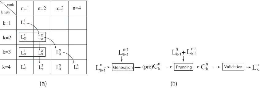
The general structure of the algorithm is that it generates first the frequent msps of rank 1

(L1

1, L12, L13, . . .), using an algorithm for mining (simple) sequential patterns (for instance, the

algo-rithm GSP ([Agrawal and Srikant 1996])). Then, for each rankn, the algorithm generates iteratively

the sets Cn

k of candidate msps of length k ≥ n. For the initial case k = n, Cnn is generated from

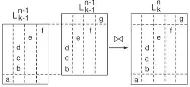
Lnn−−11, which has been generated in the previous step corresponding to rankn−1. For the casek > n, the setCkn (containing the candidatemsps of lengthkand rankn) is generated fromL

n−1

k−1 andL

n k−1

which have been generated in previous steps. The supports for these candidatemsps are computed

through a pass over the dataset. At the end of the pass, the set Lnk (the candidate msps which are

actually frequent) is computed. Thesemsps become the seed for the next passk+ 1. In Figure 5(a),

we illustrate how the setLnk is obtained from previous steps and in Figure 5(b), we illustrate the whole

mining process.

rank length

k=1 k=2 k=3

k=4

n=1 n=2 n=3 n=4 L11

L12

L13

L14 L22

L23

L24 L33

L34 L 4 4

(a)

L

nk-1 Generation

L

n-1k-1

(pre)

C

nk Prunning

L

n-1k-1

C

nk

L +

nk-1

L

nk

Validation

(b)

Fig. 5:Ln

k is obtained fromL n₋1

k₋1 andL

n k₋1

The algorithm SM is given in Figure 6. In the pass where frequentmsps of lengthkand ranknare

generated, the algorithm first generates the setCn

k, the candidatemsps (steps3.2and3.6.2). After

that, themsps that contain msps not in Ln_k−−₁1 and Ln

k−1 are pruned from Ckn. This is so because,

according to Proposition 2.1, thesemsps have no chance to be frequent (steps3.3,3.6.3and3.6.4). After the pruning phase, the supports of the candidates are computed through a pass over the dataset

(steps3.4and3.6.5). In paragraph 4.1, we show in detail how candidatemsps inCn

k are built from

the setsLnk−−11 andLnk−1 that have been calculated in previous steps.

4.1 Candidate Generation

Now, we show how to generate potentially frequentmsps in Σn

k (recall that Σnk denotes the set ofmsps

of ranknand lengthk). In this construction, we suppose that the columns of eachmsp σ∈Σn

k are

ordered by an ordering which is naturally induced by the ordering over time. For instance, in Figure

7(e) we have a non orderedmsp (left) and the samemsp where columns have been ordered (right).

We use the following notation in the sequel: if σ∈ Σn

k then σ and σdenote the multi-sequences

Input:(α: minimum support, N: number of data multi-sequences, D: dataset)

1. n= 1;k= 0;

2. Repeat 2.1k=k+ 1;

2.2L1

k= frequent sequences of rank 1 and lengthk(uses GSP)

UntilL1

k=∅;

3. Repeat

3.1n=n+ 1; k=n;

3.2Cn

n=L

n₋1

n₋11L

n₋1

n₋1 (New candidate msp’s of ranknand lengthnare generated from Ln−1

n₋1)

(For details on the operator1, see Section 4.1);

3.3 deleteall candidatesσ∈Cn

n such that∃τ⊆σ,τ∈Σ n₋1

n−1andτ /∈L

n₋1

n−1(pruning); 3.4 ForeachgroupginDdo

Increment the count of all candidatemsp’s inCn

n that are contained inS(g);

3.5Ln

n= candidates inCnnwith count≥αN;

3.6 Repeat

3.6.1k=k+ 1;

3.6.2Cn k = (L

n₋1

k₋1 1L

n₋1

k₋1)∪(L

n k−11L

n k−1)∪(L

n₋1

k₋11L

n k−1)∪(L

n k−11L

n₋1

k₋1) (New candidate msp’s of ranknand lengthkare generated

fromLn−1

k−1 andL

n

k₋1 See Section 4.1 for details);

3.6.3 deleteall candidatesσ∈Cn

k such that∃τ⊆σ,τ∈Σ n₋1

k−1 andτ /∈L

n₋1

k−1;

(pruning 1)

3.6.4 deleteall candidatesσ∈Cn

k such that∃τ⊆σ,τ∈Σ n

k−1 andτ /∈L

n k−1;

(pruning 2)

3.6.5 ForeachgroupginDdo

Increment the count of all candidatemsp’s inCn

k that are contained inS(g);

3.6.6Ln

k= candidates inC n

k with count≥αN;

UntilLn k=∅;

UntilLn n=∅

Fig. 6: Algorithm SM

As we can see in line3.6.2of Algorithm SM, there are four possibilities to obtain a candidate in

Cn k:

(1) by joining twomsps ofLn_k−−1₁, (2) by joining twomsps ofLn

k−1,

(3) by joining anmsp ofLn_k−−₁1 with anmsp ofLn k−1, and (4) by joining anmsp ofLnk−1 with anmspof L

n−1

k−1.

Figure 7 gives the conditions for twomsps being joinable (below each figure) as well as the result of the join operation, in the four cases.

The following theorem, whose proof can be found in Appendix A.1, guarantees that: (1) all frequent msps of Σn

k are included inC n

k and (2)C

n

k is minimal, in the sense that it contains only the potentially

frequentmsps of Σn k:

Theorem 4.1 For alln, k,1≤n≤k, we have: (1)Ln k ⊆C

n

k. (2) Ifσ∈Σ n

k and there exists τ⊆σ,

τ6=σ, such thatτ is not frequent, thenσ6∈Cn k.

4.2 Support Counting

In order to reduce I/O operations over the dataset and compute the support of eachmsp in Cn

k by

executing only one pass over the dataset, we find all candidates σ which are included in S(g), for

each data multi-sequenceS(g). In order to reduce the number of candidates which have to be tested

a b c d e f g b c d e f a b c d e f g Ln-1_k-1 L

n-1

k-1 L

n k

Case 1: if we eliminate the first column of σand last column ofτthen the resultingmsps are identical.

a b c d e f g b c d e f a b c d e f g

Lnk-1

Lnk-1 Lnk

Case 2a:σandτare identical.

a b c d e f g b c d e f a b c d e f g

Lnk-1

Lnk-1 Lnk

Case 2b:σandτare identical after shifting the colomns ofτone place to the right.

a b c d e g b c d e f a b c d e f g f

Ln-1k-1

Lnk-1 L

n k

Case 3: σandτ are identical and the last column ofτ

oonly contain the symbol⊥.

a b c d e f g b c d e f a b c d e f g

Lnk-1

Ln-1k-1 Lnk

Case 4: The first column ofσonly contains the symbol

⊥andσis identical toτafter shiftingσone place to the left.

0

B B @

d ⊥ ⊥

⊥ c ⊥

⊥ ⊥ b

⊥ ⊥ a

1 C C A → 0 B B @

⊥ ⊥ d

⊥ c ⊥

b ⊥ ⊥

a ⊥ ⊥

1

C C A

(e) Anmsp and its ordered version

Fig. 7: Joiningmsps

[Agrawal and Srikant 1995] for counting the support of sequences, by storing the set of candidatemsps Ckn in aset ofhash-trees. We omit these technical details here.

5. EXPERIMENTAL RESULTS

To evaluate the performance of the algorithms SM and PM, we ran several experiments using synthetic datasets. Our experiments have been run on a Pentium 4 of 2.4 GHz with 1GB of main memory and running Windows XP Professional.

5.1 Synthetic Data

We have developed a synthetic data generator using the idea described in [Agrawal and Srikant 1995] for the synthetic data-sequences generator. Our generator produces datasets of multi-sequences in accordance with the input parameters as shown in Table 1.

frequent multi-sequences (|R|) was set to 3 and the average length of potentially frequent

multi-sequences (|S|) was set to 4. Table 2 summarizes the dataset parameter settings. The dataset

D4-G4-C6, for instance, keeps 4000 groups with average number of clients per group equal to 4 and the average number of transactions per client equal to 6.

Table 1: Parameters used in the Synthetic Data Generator

|D| Number of groups (size of dataset) - in ’000s

|G| Average number of customers per group

|C| Average number of transactions per customer

|R| Average rank of potentially frequentmsp’s

|S| Average length of potentially frequentmsp’s N Number of items

Nm Number of maximal potentially frequentmsp’s

Table 2: Synthetic Datasets - Parameter Settings

Name |D| |G| |C| Size MB

D2-G4-C3 2 4 3 1.06

D2-G4-C6 2 4 6 2.09

D2-G6-C3 2 6 3 1.57

D4-G4-C6 4 4 6 4.19

5.2 Performance Analysis

Figure 8 shows the execution times of algorithms SM and PM for the four datasets given in Table 2 as the minimum support decreases from 1% to 0.25%. As expected, the execution times for both algorithms increase. PM performs worse than SM for low support levels, mainly because more patterns of large ranks are generated in the generation phase of PM. This set is more refined in SM algorithm

because the generation and pruning of the candidatesmsps are achieved without decomposing them

into the shape-sequences and item-sequences.

Both algorithms present a similar performance for high support levels. The reason is that, in this case, the generated patterns have small rank (usually less than 4) and most of the execution time is spent during the first iteration, which is the same for both algorithms.

5.3 Scale-up

We present some results regarding scale-up experiments for PM and SM. Other scale-up experiments have also been performed and similar results were obtained. Figure 9 shows how SM and PM scale up as the number of data multi-sequences (|D|) increases from 1000 to 5000. We show the results for

the datasets Dx-G3-C3 (x= 1, . . . ,5) and a minimum support set to 0,15%. The figure shows that

SM scales more linearly than PM with respect to the number of data multi-sequences.

Figure 10 shows how both algorithms scale up as the number of clients per group (|G|) increases

from 3 to 8. The datasets used were D2-Gx-C3 (x= 3, . . . ,8), for which the minimum support was

set to 0,25%.

Fig. 8: Execution times: Synthetic Data

Fig. 9: Scale-up w.r.t to data multi-sequences Fig. 10: Scale-up w.r.t. clients per group

6. ONGOING AND FURTHER RESEARCH

The two algorithms proposed in this article are designed to produce all frequent multi-sequential

patterns, regardless to users’ specific interests. At the present time, we are investigating constraint-based methods for restricting the candidate search space. Often, users require richer mechanisms for specifying patterns of interest, rather than the simple mechanism provided by minimum support.

expression as input, which aims at capturing the shape of patterns he/she is interested in discovering. The automaton associated to this regular expression is incorporated into the mining process that outputs the sequential patterns exceeding a minimum support threshold and which are accepted by

the automaton. We are investigating the introduction of regular expression restrictions overmsps and

the development of algorithms to minemsps satisfying such restrictions.

Another direction for future research concerns performance comparison between our Apriori-based method SM and methods for first-order sequential pattern mining based on Inductive Logic Program-ming. We intend also to validate our mining algorithms over real datasets.

REFERENCES

Agrawal, R. and Srikant, R. Mining Sequential Patterns. InProceedings of the International Conference on Data Engineering. Taipei, Taiwan, pp. 3–14, 1995.

Agrawal, R. and Srikant, R. Mining Sequential Patterns: Generalizations and Performance Improvements. In Proceedings of the Fifth Int. Conference on Extending Database Technology. Avignon, France, pp. 3–17, 1996. Berger, G. and Tuzhilin, A. Discovering unexpected patterns in temporal data using temporal logic. Information

Systems Working Papers Series, 1999.

Bettini, C.,Wang, X. S.,and Jajodia, S.Testing complex temporal relationships involving multiple granularities and its application to data mining (extended abstract). InProceedings of the Fifteenth ACM SIGACT-SIGMOD-SIGART Symposium on Principles of Database Systems. Montreal, Canada, pp. 68–78, 1996.

Das, G.,ip Lin, K.,Mannila, H.,Renganathan, G.,and Smyth, P.Rule discovery from time series. InProceedings of the 4th International Conference of Knowledge Discovery and Data Mining. AAAI Press, New York City, USA, pp. 16–22, 1998.

Garofalakis, M. N.,Rastogi, R.,and Shim, K.Spirit: Sequential pattern mining with regular expression constraints. InProceedings of the International Conference on Very Large Databases. Edinburgh, Scotland, pp. 223–234, 1999. Han, J.,Pei, J.,Mortazavi-Asl, B.,Chen, Q.,Dayal, U.,and Hsu, M.-C. Freespan: frequent pattern-projected

sequential pattern mining. In Proceedings of the sixth ACM SIGKDD International Conference on Knowledge Discovery and Data Mining. Boston, USA, pp. 355–359, 2000.

Jacobs, N. and Blockeel, H. From shell logs to shell scripts. InProceedings of the International Conference on Inductive Logic Programming. Strasbourg, France, pp. 80–90, 2001.

Joshi, M.,Karypis, G.,and Kumar, V. A universal formulation of sequential patterns. Tech. rep., Technical Report 99-021, Department of Computer Science and Engineering, University of Minnesota, USA, 1999.

Lee, S. D. and Raedt, L. D. Constraint Based Mining of First Order Sequences in SeqLog. In Proceedings of the Workshop on Multi-Relational Data Mining. ACM SIGKDD, Alberta, Canada, 2002.

Lu, H.,Feng, L.,and Han, J.Beyond intratransaction association analysis: mining multidimensional intertransaction association rules.ACM Transactions on Information Systems18 (4): 423–454, 2000.

Mannila, H.,Toivonen, H.,and Verkamo, A. I. Discovery of frequent episodes in event sequences. Data Mining and Knowledge Discovery1 (3): 259–289, 1997.

Masson, C. and Jacquenet, F.Mining frequent logical sequences with spirit-log. InProceedings of the International Conference on Inductive Logic Programming. Sydney, Australia, pp. 166–181, 2002.

Padmanabhan, B. and Tuzhilin, A.Pattern discovery in temporal databases: A temporal logic approach. In Proceed-ings of the Second International Conference on Knowledge Discovery in Databases. Portland, USA, pp. 351–354, 1996.

Pinto, H.,Han, J.,Pei, J.,Wang, K.,Chen, Q.,and Dayal, U. Multi-dimensional sequential pattern mining. In Proceedings of the Tenth International Conference on Information and Knowledge Management. Atlanta, USA, pp. 81–88, 2001.

Zaki, M. J.Spade: an efficient algorithm for mining frequent sequences.Machine Learning Journal vol. 42, pp. 31–60, 2001.

A. PROOFS

A.1 Proof of Theorem 4.1

(1) Letσ∈Ln

k. We suppose the columns ofσ are ordered (See Figure 7 (e)). Forn= 1, the result

is verified, because the candidate generation procedure used in algorithm Apriori-All is correct, i.e., the set of candidates always contains all frequent sequences. Forn=k= 2, the result is also verified because, asσ∈L22, themsps{hσ11i}and{hσ22i} are inL11. So, by construction ofC22, it is clear that L2

2⊆C22. Letn, k be such that 2≤n≤kandk≥3. We have the following cases to consider:

—The (unique) item of line 2 is placed in column 1 and

(a) there exists an item in columnnplaced in a linei, withi < k: in this case,σ∈Ln k 1

n k L

n k,

(b) columnncontains only one item, which is placed in linek: in this case,σ∈L_kn₋−₁11nk L n k.

—The (unique) item of line 2 is placed in column 2 and

(a) there exists an item in columnnplaced in a linei, withi < k: in this case,σ∈Ln k 1nk L

n−1

k−1, (b) columnncontains only one item, which is placed in linek: in this case,σ∈L_kn₋−₁11nk L

n−1

k−1.

(2) Sinceτ⊆σandτ6=σ,τ ∈Σm

p withm < norp < k. Then:

—Letm < nandm≤p≤k. In this case,τ is obtained by deleting at least one column ofσand one of the lines corresponding to the items in this column. Sop < k. We can suppose, without loss of

generality, that only one column has been deleted, i.e. m=n−1. We have thatτ is contained in

anmsp τ′ ∈Σn−1

k−1, such thatτ

′ _{⊆σ. Since τ is not frequent, thenτ}′ _{is not frequent as well, i.e.,}

τ′_6∈Ln−1

k−1. Then, by construction of themsps inC

n k,σ6∈C

n k.

—Letm=n andn ≤p < k. In this case, τ is obtained by deleting at least one line ofσ. We can suppose, without loss of generality, that only one line has been deleted. Thus,τ ∈Σn

k−1. Sinceτis not frequent, i.e. τ6∈Ln

k−1, by construction of themsps inC

n k,σ6∈C

n

k. 2

A.2 Proof of Theorem 3.1

The proof follows from the proof of Theorem 4.1 just above. This is so because theJ oinS operation

between shape-sequences is defined in such a way that:

Πs((Lnk−−111L

n−1

k−1)∪(L

n−1

k−1 1L

n

k−1)∪(L

n k−11L

n

k−1)∪(L

n k−11L

n k−1)) = J oinS(Πs(Lnk−−11),Πs(Lnk−−11))∪J oinS(Πs(Lnk−−11),Πs(Lnk−1))∪