Asymptotic Distributions of Estimators of Eigenvalues and Eigenfunctions in Functional Data

Asymptotic Distributions of Estimators of Eigenvalues

and Eigenfunctions in Functional Data

P. Hall

1

and S.M.E. Hosseini-Nasab

2,*

1_{Department of Mathematics and Statistics, The University of Melbourne, Melbourne, Australia} 2_{Department of Statistics, Faculty of Basic Sciences, Tarbiat Modares}

University, Tehran, Islamic Republic of Iran

Received: 26 November 2007 / Revised: 5 November 2008 / Accepted: 16 November 2008

Abstract

Functional data analysis is a relatively new and rapidly growing area of

statistics. This is partly due to technological advancements which have made it

possible to generate new types of data that are in the form of curves. Because the

data are functions, they lie in function spaces, which are of infinite dimension. To

analyse functional data, one way, which is widely used, is to employ principal

component analysis, allowing finite dimensional analysis of the problem. The

authors gave stochastic expansions of estimators eigenvalues and eigenfunctions,

providing not only a new understanding of the effects of truncating to a finite

number of principal components, but also pointing to new methodology, such as

simultaneous and individual bootstrap confidence statements for eigenvalues and

eigenfunctions. The expansions explicitly include terms of sizes

n

−1/2

,

n

−1

, and a

remainder of order

n

−3/2

, where

n

denotes sample size. The terms of size

n

−1/2

are

related to limit theory. Because for many situations, the exact statistical properties

of the eigenvalues and eigenfunctions estimators are not directly obtainable, the

way by which we can approximate their distributions is of interest in practice. In

this paper, we discuss asymptotic results for eigenvalues and eigenfunctions. The

work shows that eigenvalue spacings have only a second-order effect on

properties of eigenvalue estimators, but a first-order effect on properties of

eigenfunction estimators.

Keywords: Eigenfunction; Eigenvalue; Functional data analysis; Hilbert-Schmidt operator; Stochastic expansion

*_{Corresponding author, Tel.: +98(21)82884480, Fax: +98(21)88009730, E-mail: [email protected]}

Introduction

In recent years, there has been substantial interest in research on functional data analysis. Application of new technologies allows data analysts to access a new kind of data which are functions. Similar to classical

Statistical methodologies which are finite-dimensional in conventional statistical settings, become infinite-dimensional in the context of functional data. Therefore, they challenge classical methods of data analysis and need theoretical justification.

We may describe PCA for FDA as a generalization of classical PCA so that matrix-based arguments are changed to operator-based ones in function spaces such as Hilbert spaces. However, theoretical treatments for FDA are not as easy as we are thinking about in that way. High dimensionality of the problems in this field, alter substantially both numerical and theoretical properties of statistical methodology. See, for example, [16,17]. Some theoretical justification for PCA in functional data analysis is provided by limit theory. See, for example, [14] and [8].

1. What Are Functional Data?

One of the aspects of functional data is to show changes over time (the “age” effect), separated from the effects caused by differences among subjects which are chosen from the population for the study. This is due to the nature of the collected data, consisting of repeated measurements of subjects through time. Unlike cross-sectional studies, in which we measure a single quantity for each object, here we are able to use the capacity of data to explore the “age” effect by analyzing the data. Separation of changes over time within objects from those among them can be beneficial for revealing useful characterizations of the population from which the sample was drawn. In a sample like X t1( ), ,L X tn( ), the former variation refers to the variablet, time, which belongs to an interval, say [ , ]a b , and the second can be seen through the essential randomness of X , in which for a certain time, we have different values of X when running from the first individual (X t1( )) to the last one in the sample (X t_n( )). In cross-sectional data, however, we can see the differences among individuals by measuring a quantity over sampled individuals, showing

1, 2, , n

X X L X .

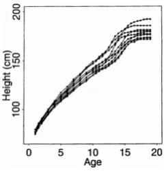
Figure 1 shows the heights of ten boys, obtained by measuring each boy at 29 different points of time ([25], page 2). For each boy, measurement was begun at age two and continued annually until age ten, after which it was done biannually for all boys. Therefore, we have 29 records for each person, which can be assumed as a continuous function due to the nature of growth. As the graph shows, it can be easily recognized that the sign of almost all boys' height accelerations tend to change at some points (ages), especially at 12, 14, and 16. This might be due to pubertal effects on their growth.

However, the effect is not the same for all boys, and differs in the timing and the intensity. To explore the “age” effect, one can be benefited by using tools for investigating behavior of functions, such as obtaining the acceleration curves by estimating the D2_Height i

from the data. Thus, thinking of records as curves rather than vectors of observations in discrete time enables us to employ derivatives for investigating the “age” effect in functional data ([25], page 2).

2. Principal Component Analysis for Functional Data

Classical principal component analysis (PCA) is amongst the oldest of the multivariate statistical methods of data reduction. A Multivariate Analysis problem could start out with a substantial number of correlated variables. In such situations, using PCA, we can reduce the number of the variables to a lesser number of constructed variables from the original data that are uncorrelated and account for most of the variation in the original data set. It helps us to understand the underlying structure of the data. For this reason, PCA has found application in fields such as signal processing, face recognition, image compression and so on ([21]). Similarly, PCA is widely used in the study of functional data, since it allows finite-dimensional analysis of a problem that is intrinsically infinite-dimensional.

Early work on PCA for FDA includes that of [4,24,27,23,29,30]. Accounts in monographs include those of [25], especially Chapter 6, and [26]. Work of [14,7,3,19,22], for example, addresses empirical basis function approximation and approximations of covariance operators.

Recent work includes contributions to techniques for functional PCA (see e.g. [1,2,6,9-13,15,18,20].

2.1. Kernel for Principal Component Analysis

Let X denote a random function, or equivalently a stochastic process, defined in the interval I = [0,1] and satisfying ₍ 2_{) <}

IE X ¥

ò

. Put m =E X( ), a conven-tional function. The principal component expansion of X -m may be constructed via the covariance function,

[

]

( , ) = { ( ) ( )}{ ( ) ( )} .

K u v E X u -mu X v -mv

We interpret K as the kernel of a mapping, or operator (also denoted by K ), on the space L I2( ) of square-integrable functions from I to the real line. It takesy ÎL I₂( ) to Ky, where

( )( ) = ( , ) ( ) . I

Ky u

ò

K u v y v dv (1)

We may write

=1

( , ) = _{j j}( ) _j( ), j

K u v

å

¥q y uy v (2)

where q q1³ 2 ³L³0 is an enumeration of the eigenvalues of K , and the corresponding orthonormal eigenfunctions arey y₁, ₂,_K.

The yj’s are sometimes called the principal component functions of K .

2.2. Empirical Principal Components

Suppose we are given a set X = {X1, ,K Xn} of independent random functions, all distributed as X . The standard empirical approximation to K u v( , ) is

=1 1

ˆ ( , ) = n { i( ) ( )}{ i( ) ( )}, i

K u v X u X u X v X v

n

å

-

-where ₌ 1 i i

X n-

å

X _.

Analogously to (1) and (2), we can write the kernel operator Kˆ , on the space L I2( ) as follows:

ˆ _ˆ ˆ _ˆ

( )( ) = ( , ) ( ) , I

Ky u

ò

K u v y v dv

and the empirical spectral decomposition

=1 ˆ

ˆ_{( , ) = ˆ ( )ˆ ( ),} j j j j

K u v

å

¥q y uy v

where qˆ1³qˆ2 ³L³0 is an enumeration of the eigenvalues of Kˆ , and the corresponding orthonormal eigenfunctions arey yˆ ˆ₁, ₂,_K.

2.3. Karhunen-Loève Expansion

An expansion of the function X -m with respect to the orthonormal basis yj (in L I2( ) sense) is its Karhunen-Loève expansion:

=1

( ) ( ) = _{j j}( ), j

X u -mu

å

¥x y u (3)

where the principal components x x1, ,2 K are given by

I

= ( )

j X j

x

ò

-m y . As regards the kernel K u v( , ), it follows that

I I

( _{j k}) = _j( ) ( , ) _k( ) = _{j jk}, E x x

ò ò

y u K u v y v du dv q d (4)

where djk is the Kronecker delta (recall that the 1/2 j

q

are eigenvalues and 1/ 2 j

y are the corresponding orthonornal eigenfunctions of the operator K ). Equation implies that the random variables x_j are uncorrelated, with zero means and variance

2 = ( ) j E j

q x . Moreover, 2

1 IE X( -m) =

å

j³qj <¥

ò

.

We call the expansion the Karhunen-Loève expansion of X -m. It is also known that if the kernel K u v( , ) is a continuous function on I I´ , then the series on the right-hand side of converges uniformly to X u( )-m( )u

(Theorem 1.5 of [8]). However, the L₂ convergence of the series to X u( )-m( )u , satisfied by the condition

2 IE X[( -m) ] <¥

ò

.

Also, in regard to ˆ ( , )K u v as the standard empirical approximation to K u v( , ), we write

=1 ˆ ˆ

= ,

i ij j

j

X -X

å

¥x y

where

I

ˆ _{= ( )ˆ}

ij Xi X j

x

ò

- y is the j th empirical principal component of X_i. In analogy to (4),

I I =1

1 _{ˆ ˆ ˆ ˆ ˆ ˆ}

= ( ) ( , ) ( ) = . n

ij ik j k j jk

i

u K u v v du dv n

å

x x

ò ò

y y q d

[16,17] developed rigorous arguments, based on arguments from operator theory, that derive stochastic expansions for eigenvalues and eigenfunctions estimators as follows.

2.4. Stochastic Expansions for Eigenvalues and Eigenfunctions

and eigenfunctions which explicitly include terms of sizes _n-1/2 _{and n}-1_{, where n denotes sample size, and} a remainder of order _n-3/2_{. This work shows that} eigenvalue spacings have only a second-order effect on properties of eigenvalue estimators, but a first-order effect on properties of eigenfunction estimators.

Take I to be the unit interval. Put A =X -E X( ) and assume that

(a) for allC >0 and some e >0,

| ( ) | < ,

sup C

t

E X t

Î

¥

I

,

[{| | | ( ) ( ) |} ] < ;

sup C

s t

E s t -e X s X t

Î

- - ¥

I

(5)

(b) for each integerr≥1, 2 , r ( ) r

j E _IA j

q - y

ò

is bounded uniformly inj. For example, (5) holds for Gaussian processes with Hölder-continuous sample paths.

Recall that the eigenvalues of the covariance operator

K are ordered so that q q1³ 2 ³K³0. Let z Îj (0,1) denote the infimum of 1 (- q qk / j) over K such that

< k j

q q , and let n Îj (0,1) denote the infimum of (q q -k / j) 1 over k such that qk >qj . Define

2 2

ˆ ˆ

|||K -K ||| = (

ò

K -K) , and put rj =mink¹j|qj -qk |, and sj =supu|yj( ) |u .

Theorem 1. If (5) holds, then for eachj for which 1

ˆ _{min( , ),}

2 j j j

K K- £ q z n (6)

ˆ ( )_j t _j( )t

y -y = 1/ 2 1

:

( _{j k}) _k( ) _{j k} k k j

n- q q -y t Zy y

¹

-å

ò

1 2 2

:

12 _j( ) ( _{j k}) ( _{j k}) k k j

n-y t q q - Zy y

¹

-

å

-

ò

1 1

:

( ){( )

k j k

k k j

n- y t q q -¹

+

å

-1

:

( j ) ( j )( k )

j

Z Z

q q - y y y y

¹

´

å

- _l

ò

_l

ò

_l

l l

2 3/ 2

(qj qk) ( Zy yj j)( Zy yj k)} O np( ),

-

-- -

ò

ò

+ (7)

1/ 2 1

ˆ ₌

j j n Z j j n

q _-q - y y ₊

-ò

1 2 3/2

:

( _{j k}) ( _{j k}) _p( ), k k j

Z O n

q q - y y

-¹

´

å

-

ò

+ (8)

where the absolute values of the “ ₍ 3/2₎ p

O n- _”

remainders on the right-hand sides of (7) and (8) are each bounded above by 3/2 _{(1 )} 1/ 2 3 1/ 2

nj j j j j

n- U -z - r q- - s , where the random variables Unj satisfy

, 1 ( ) <

sup C

nj

n j³E U ¥ for each C > 0. In the case of (7), this bound is also valid uniformly in t. Moreover, the “ ₍ 3/2₎

p

O n- _{” remainders on the right-hand sides of (8)} are bounded above in the L2 metric by n-3/2Unjrj-3, where theU_nj have the same properties as before.

Proof: See [16].

Using the stochastic expansions given in and, and their properties, here we discuss the weak convergence results for estimators of eigenvalues and eigenfunctions. Lemma 1. If the random process X t( ) satisfies the following condition:

for allC > 0 and somee >0,

| ( ) | < ,

sup C

t

E X t

Î

¥

I

,

[{| | | ( ) ( ) |} ] < ,

sup C

s t

E s t -e X s X t

Î

- - ¥

I

(9)

then _{Z u v( , ) =n}1/2_{(K K u v}ˆ_{- )( , )®z( , )u v in} distri-bution, wherez is a Gaussian process.

Proof: See the appendix.

The stochastic expansions for eigenvalues and eigenfunctions given in (7) and (8) are of intrinsic interest. They can be used as the foundation for theory in a particularly wide range of settings, for example bootstrap methods for confidence intervals for eigenvalues and eigenfunctions ([16]). However, in order to develop informative theory about the performance of such methodologies, we need a concise account of the accuracy to which qˆ_j and yˆ_j approximate q_j andy_j, respectively. That account can be easily provided using properties of the expansions. Moreover, the problem of determining estimator accuracy, uniformly over many components, prompts consideration of explicit uniform bounds that are obtainable via the mathematical theory of infinite-dimensional operators ([17]).

The weak limit of Z , z , is a bivariate Gaussian process with mean zero and the covariance function

( , , , ) cov{ ( , ), ( , )}

{ ( ) ( ) ( ) ( )}

( , ) ( , ), C u v s t u v s t

E Y u Y v Y s Y t

K u v K s t

z z

=

=

the Karhunen-Loève expansion Y u( ) = _j=1x yj j( )u ¥

å

,

where I = j Y j

x

ò

y , we have:

( , , , )

C u v s t

1 4 1 2 3 4

=1 =1

1 4

( j j ) j ( ) j ( ) j ( ) j ( ) j j

E x x y u y v y s y t ¥ ¥

=

å å

_{K K}

1 2 1 1 2 2

=1 =1 1 2

( ) ( ) ( ) ( ),

j j j j j j

j j

u v s t

q q y y y y

¥ ¥

-

å å

(10)

where we have used the fact that ₍ 2 _{) =} j_k j_k E x q . If the absence of correlation among the x_j's is replaced by independence, only for the purpose of calculating the expected values of products of four of the variables xj, then the first series on the right-hand side of (10) can be written as

1 4 1 2 3 4

=1 =1

1 4

( j j ) j ( ) j ( ) j ( ) j ( ) j j

E x x y u y v y s y t ¥ ¥

=

å å

K K

4

=1

( )_{j j}( ) _j( ) _j( ) _j( ) j

E x y uy v y sy t

å

1 2 1 1 2 2

1 2

{ ( ) ( ) ( ) ( )

j j j j j j

j j

u v s t

q q y y y y

¹

+

åå

1( ) 1( ) 2( ) 2( ) j u j s j v j t

y y y y

+

1( ) 1( ) 2( ) 2( )}. j u j t j s j v

y y y y

+

Therefore, ( , , , )

C u v s t

4 2

=1

{ ( )j j} j( ) j( ) j( ) j( ) j

E x q y uy v y sy t

¥

=

å

-1 2 1 1 2 2

1 2

{ ( ) ( ) ( ) ( )

j j j j j j

j j

u s v t

q q y y y y

¹

+

åå

1( ) 1( ) 2( ) 2( )}. j u j t j s j v

y y y y

+ (11)

Under the assumption that random processes X is a Gaussian processes, (i.e. the variables x_j are independent and jointly normally distributed, rather than merely uncorrelated, and with zero kurtosis),

4 2

( ) = 3j j

E x q . In this situation, the asymptotic covariance function is simplified as follows:

( , , , )

C u v s t

1 2 1 2 1 2

1 2

{ ( ) ( ) ( ) ( )

j j j j j j

j j

u v s t

q q y y y y

¹

=

åå

1( ) 2( ) 2( ) 1( )} j u j v j s j t

y y y y

+

2

=1

2 j j( ) j( ) j( ) j( ). j

u v s t

q y y y y

¥

+

å

(12)

Results

For many situations, the exact statistical properties of the eigenvalues and eigenfunctions estimators are not directly obtainable. Therefore, the way by which we can approximate their distributions is of interest in practice. In this section, we discuss asymptotic results for eigenvalues and eigenfunctions. The asymptotic results discussed here, can be used to a construct confidence interval for q_j, helping to qualify the amount of variability that can be explained by the jth principle component. Also, an asymptotic confidence interval for

j

y provides information about the likelihood that a bump on ˆy_j reflects a similar feature in the true eigenfunctiony_j.

Asymptotic Distribution of Eigenvalues and Eigenfunctions

It should be mentioned that accounts of asymptotic normality of eigenfunctions and eigenvectors and their projections have been given by [14] and [8]. In connection with the results discussed above, using the expansion (7) and (8) , the following shorter expansions can be derived:

1/2_{(ˆ ( ) ( ))}

j j

n y t -y t

1

:

( _{j k}) _k( ) _{j k p}(1). k k j

t Z o

q q -y y y

¹

=

å

-

ò

+ (13)

1/2₍ˆ _{) = (1).}

j j j j p

n q -q

ò

Zy y +o (14)

Similarly, it can be seen from equation (7) that: 2

ˆ_{j j} ||

n||y -y

2 2

:

( j k) ( j k) p(1), k k j

Z o

q q - y y

¹

=

å

-

ò

+ (15)

Results 13-15 lead directly to limit theorems for ˆy_j

and ˆq_j, as follows.

Let P_j =y_jÄy_j andQ_j= 1 : ( j k) k k k k j q q y y

-¹ - Ä

where xÄy is defined by (xÄy f) =áx f y, ñ for each f ÎE . Define the operator Fj such that it maps

Z ÎF to Q ZP_{j j} ÎF , where F , the space of all Hilbert-Schmidt operators on E with the inner product

.,.F

á ñ

1, 2 F = 1 j, 2 j E, j

T T T e T e

á ñ

å

á ñ

and the Borel field B_F .

Theorem 2. if theyj's are continuous (for each j ³1,

[0,1] j C

y Î ), then the random function 1/2_{(ˆ ( ) ( ))}

j j

n y t -y t converges weakly to a Gaussian process, Y_j( )t say, precisely;

1/2_{(ˆ ( ) ( )) ( )}

j j j

n y t -y t ® Y t =

1

:

( _{j k}) _k( ) _{j k}, in distribution k k j

t

q q -y zy y

¹

-å

ò

(16)

Proof: The proof is straightfoward. The operator F_j is linear and continuous. So, Lemma 1 implies that

( ) ( ) j Z j z

F ® F in distribution.

where the non-stationary Gaussian process Y_j( )t has zero mean and covariance function

( , ) j u v

t =

1 1

1 2 1 2

1: 1 2: 2

( j k ) ( j k ) k ( ) k ( ) k k j k k j

u v

q q - q q -y y

¹ ¹

-

-å -å

1 2

( , , , ) _j( ) _k ( ) _j( ) _k ( ) , C u v s t y u y v y s y t du dv ds dt

´

ò

where C u v s t( , , , ) was introduced in (10). After some algebraic calculations, under the assumption of independence the above formula is simplified to

2

:

( , ) = ( ) ( ) ( ).

j j k j k k k

k k j

u v u v

t q q -q q y y

¹

-å

In particular, the asymptotic variance of 1/2_{ˆ ( )} j

n y t

equals

2 2 2

:

( ) = ( , ) = ( ) ( ) .

j j j k j k k

k k j

t t t t

s t q q -q q y

¹

-å

(17)

Result (16) can be extended to a p-tuple of the ˆy_j. The p-tuple 1/2_{(ˆ ( ) ( ))}

j j

n y t -y t for 1£ £j p

converge jointly and weakly to the non-stationary Gaussian process Y₁, ,_L Y_p. In particular, for

1, 2 1

j j ³ , the two random functions

1/ 2

1 1

ˆ

( _j ( ) _j ( ))

n- y t _-y t _and 1/ 2

2 2

ˆ

( _j ( ) _j ( )) n- y t _-y t _have the asymptotic covariance function

2

, ,

1 2 1 2 1 1

: ₁

( , ) = ( ) ( ) ( )

j j j j j k j k k k

k k j

u v u v

t d q q -q q y y

¹

-å

2 ,

1 2 2 1 1 2 2 1

(d_{j j} 1)(q_j q_j )-q q y_{j j j} ( )u y_j ( ),v

+ -

-where _, 1 2 j j

d denotes the Kronecker delta. The covariance function shows that for j₁¹ j₂, the two elements 1/ 2

1 1

ˆ

( _j ( ) _j ( ))

n- y t _-y t _and 1/ 2 2 ˆ ( _j ( ) n- y t

-2( )) j t

y are not asymptotically independent.

Therem 3. in connection to (15), if (9) holds, then we have

1/2 _{ˆ , in distribution,}

j j j

n ||y -y ||®U (20)

where

2 2 2

:

= ( ) ,

j j k jk

k k j

U q q - N

¹

-å

(19)

and the random variables Njk =

ò

zy yj k are jointly normally distributed with zero mean. Morever, if the random function X is a Gaussian process then

1, 2, j j

N N _K are independent as well as normally distributed.

Proof: The proof is straightforward by using lemma1 and result (15). Note that, since 4

IE X( ) <¥

ò

,

2 2

=1 =1

( _jk) = ( _jk)

k k

E N E N

¥ ¥

å

å

2 I I

= { [E

ò ò

z( , )u v yj( )v dv du] }

2 2 IE(z )

£

òò

2 2 2

I I

=

ò ò

{ [ ( )E X u X v( ) ]-K u v( , ) }du dv

2 2

I IE X u X v[ ( ) ( ) ]du dv

£

ò ò

2 2 4

I I

= (E

ò

X ) £

ò

E X( ) < ,¥ (20)

from which it follows that the series defining 2 j

U is finite provided the eigenvalueq_j is not repeated. Result 1. It implies that

1/2₍ˆ _{) , in distribution,}

j j jj

n q -q ®N (21)

variance

2 _{= ( )}4 2_.

j E j j

g x -q (22)

An extension of the result (21) is available for anyp -tuple of the qˆ_j. The p-tuple 1/2₍ˆ ₎

j j

n q -q for 1£ £j p converge jointly to a p-variate Normal distribution. In particular, for j j₁, ₂³1, the two random quantities 1/2

1 1

ˆ ( j j )

n q -q and 1/2

2 2

ˆ ( j j ) n q -q are asymptotically distributed as a two-variate Normal distribution with the covariance

2 2

1 2 = ( 1 2) 1 2. j j E j j j j

g x x -q q

Comparing result (21) with formula (19) for the limiting distribution of 1/2 _ˆ

j j

n ||y -y ||, we see that spacings among the eigenvalues q_k impact immediately on properties of ˆy_j, through first-order terms in its limiting distribution; but impact on ˆq_j only through second-order terms. Note also , where it is clear that eigenvalue spacings affect only the term in _n-1_{, not that} in _n-1/2_.

Appendix

Proof of Lemma 1. We have

1/2 ˆ

( , ) = ( )( , )

Z u v n K K u v

-1/ 2

=1 1

= [( n i( ) ( )i ( , )) i

n Y u Y v K u v

n

å

-{ ( )X u h( )}{ ( )u X v h( )}]v

- -

-1/ 2

=1 1

= [ n _i( , ) { ( ) i

n W u v X u

n

å

-( )}{ -( )u X v ( )}],v

h h

- - (23)

where h( ) = { ( )}u E X u , Y_i =X_i -h andW u v_i( , ) = ( ) ( ) ( , )

i i

Y u Y v -K u v . The first term on the right-hand side of is the sample mean of then independent terms. Furthermore, by using the fact that X v( )

-1/ 2 ( ) =v O np( )

h - _{(Theorem 3.2.5 of [29] with tightness} of X v( ) which is discussed later), we can write

1/ 2 ( , ) = n( , ) p( )

Z u v Z u v +O n- , where Z u v_n( , ) = 1/ 2

=1 ( , ) n

i i

n-

å

W u v _.

Theorem 4. Let P_n and P be probability measures on

[0,1]

(C , )F , where C_[0,1] is the space of continuous functions on [0,1] with the uniform metric

( , ) =x y sup_t| ( )x t y t( ) |

r - , for each x y, ÎC_[0,1], and F is the s -field constructed on C_[0,1]. If the finite-dimensional distributions of P_n converge weakly to those of P, and if { }Pn is tight, then Pn converges weakly to P.

Proof: See Theorem 8.1 of [5]. ■

Using the above theorem, if X_n are random elements of C[0,1], then {Xn} is tight if { }Pn is tight, where P_n is the distribution of X_n, as we identify the finite-dimensional distribution of X_n with those of P_n

in the above theorem. Therefore, Theorem 4 is equivalent to the following argument.

If the finite-dimensional distributions of X_n

converge weakly to those of X , and {X_n} is tight, then X_n ®X in distribution. Regarding the k points

1 1

( , ), ,( ,u v _L u v_{k k}), for each point if 4 IE X( ) <¥

ò

,

then the classical Central Limit Theorem with the Slutsky Theorem (Theorem 3.3.1 and 3.4.2 of [28]) implies that, for each = 1, ,j _L k,

( , ) (1) ( , )

n j j p j j

Z u v +o ®z u v , in distribution, (24)

where z( , )u v_{j j} is the weak limit of Z u v( , )_{j j} , for each j = 1, ,L k . Now, for the k points

1 1

( , ), ,( ,u v _L u v_{k k}) in [0,1] [0,1]´ , let _{( , ), ,( , )} 1 1 u v u_kv_k

P _L

be the mapping that carries the pointh of C_{[0,1] [0,1]´} to the point ( ( , ), , ( , ))h u v_{1 1 L} h u v_{k k} of _Rk_{. Since}

( , ), ,(u v_{1 1} u_k,v_k)

P _L is continuous, we have

( , ), ,(u v_{1 1} u_k,v_k)(Zn) ( , ), ,(u v_{1 1} u_k,v_k)( )z

P _L ® P _L in distribution (Corollary 1 of Theorem 5.1 of [5]), i.e.

1 1

(Z u v_n( , ), ,L Z u v_n( ,_{k k}))®

1 1

( ( , ), , ( ,z u v _L z u v_{k k})),in distribution. (25)

(in particular, (25) follows via the Cramér-Wold device.)

Theorem 5. The sequence {X_n} is tight if it satisfies these two conditions:

(i) The sequence {Xn(0)} is tight.

2 1 2 1 1

{| n( ) n( ) | } | ( ) ( ) | ,

P X t X t l _g F t F t a

l

- ³ £ - (26)

holds for all t t₁, ₂ and n and all positive l.

Proof: See Theorem 12.3 of [5]. ■ We know that the moment condition

2 1 2 1

{| _n( ) _n( ) | } | ( ) ( ) | ,

E X t -X t g £F t -F t a (27)

implies. Furthermore, we can immediately obtain tightness of {Xn} from condition (9), (27) and Theorem 5. Also, for some = 2g k , where k ³1 is an integer, using Rosenthal's inequality for fixed

, , , [0,1]

u v s tÎ results in

1/ 2 1/2

=1 =1

[| n _i( , ) n _i( , ) | ]

i i

E n-

å

W u v _-n-

å

W s t g

2

=1

= k | n{ ( , ) ( , )} |k

i i

i

n E-

å

W u v _-W s t

2 1

=1

{n | ( , ) ( , ) |

k k

i i

i

C n_g - E W u v W s t

£

å

-2

=1

( n | ( , ) ( , ) | ) }k

i i

i

E W u v W s t

+

å

-2 | ( , ) ( , ) | ,

C E W u vg W s t g

£ - (28)

and

| ( , ) ( , ) | =

E W u v -W s t g

|{ ( ) ( ) ( ) ( )} { ( , ) ( , )} |

E Y u Y v -Y s Y t - K u v -K s t g

3 ( | ( ) ( ) ( ) ( ) |

C E Y u Y v Y s Y t g g

£

-| ( ) ( ) ( ) ( ) | )

E Y u Y v Y s Y t g

+

-4 | ( ) ( ) ( ) ( ) | ,

C E Y u Y v Y s Y t g g

£ - (29)

whereC1g, C2g, C3g andC4g are constants depending

only on g, g , andW andY denote a genericW_i and

i

Y , respectively. Also,

[| ( ) ( ) ( ) ( ) | ]

E Y u Y v -Y s Y t g

[| ( )( ( ) ( )) ( )( ( ) ( ) | ]

E Y u Y v Y t Y t Y u Y s g

= - +

-{ [| ( ) | | ( ) ( ) | ]

C E Y ug g Y v Y t g

£

-[| ( ) | | ( ) ( ) | ]}

E Y t g Y u Y s g

+

-2 1/ 2 2 1/2

{( [| ( ) | ]) ( [| ( ) ( ) | ])

Cg E Y u g E Y v Y t g

£

-2 1/ 2 2 1/2

( [| ( ) | ]) ( [| ( )E Y t g E Y u Y s( ) | ]) },g

+ - (30)

where Cg is a constant depending only on g. If

condition (9) holds, then (28)-(30) imply that for each two points ( , ),( , ) [0,1] [0,1]u v s t Î ´ ,

1/ 2 1/2

=1 =1

[| n i( , ) n i( , ) | ]

i i

E n-

å

W u v _-n-

å

W s t g

{| | | | },

C v t a u s a g

£ - + - (31)

where g can be chosen such that a e g= > 2. Hence, using Markov's inequality, for each l> 0, each two points ( , ),( , )u v s t Î ´I I and all n we have

1/2 1/ 2

=1 =1

(| n ( , ) n ( , ) |> )

n i i

i i

P n-

å

W u v _-n-

å

W s t l

{| | | | }.

C g v t a u s a gl

-£ - + - (32)

The proof of the above theorem, given by [5], with condition (32) instead of (26) may be followed to show that 1/ 2

=1 ( , ) n

i i

n-

å

W u v is tight. To appreciate why, fix

n, d , j and k , then for a positive integer m

consider the random variables

1/ 2

=1

= n ( i( , )

i

n W j k

m m

k -

å

d₊ d d₊ d

l l l

( 1) ( 1)

( , )),

i

W j k

m m

d - d d - d

- + l + l

for _l=1, ,_L m. The random variables k_l with

=1

= k

k

S

å

_l k_l satisfy

< = s r

r s

S S k

£

-

å

_l

l

1/ 2

=1

= n ( i( , )

i

s s

n W j k

m m

d d d d

-

å

_{+ +}

( , )).

i

r r

W j k

m m

d d d d

- + +

So, for 0£ £ £r s m andl> 0 we have

<

(| _{s r} | ) = (| | ) r s

P S S l P k l

£

- ³

å

_l ³

l

( ) ( )

[( s r ) ( s r ) ]

C

m m

g a a

g

d d

l- -

-£ +

1 1

< <

[( ) ( ) ]

r s r s

Cgl-g dm- a dm- a

£ £

£

å

+

å

,

Cgl d-g a

£

where we have used (32) to obtain the first inequality above. By using Theorem 12.2 of [5], we have

1/2

0 ₌₁

(max| ( ( , )

n

i

m _i

P n W j k

m m

d d d d

-£ -£l

å

+ +

l l

( , )) |> ) , i

B

W j k a

g

d d e d

e

- £

where B depends on g and a (B =B_{g a,} ). Since the

i

W for each 1£ £i n are continuous functions, if

m® ¥ we have

1/2

( , ) ( , ) < =1

( sup | n ( _i( , ) u v j k E i

P n W u v

d d d

--

å

|| ||

( , )) |> ) . i

B W jd dk e _gda

e

- £ (33)

where .|| ||_E denotes the Euclidian norm in _R2_{. If d}-1 is integer, the above inequality leads to

1/ 2

( , ) ( , ) <

1 1 =1

< <

( sup | n ( i( , )

u v j k E i j k

P n W u v

d d d d d

--

-å -å

å

|| ||

2 ( , )) |> ) . i

B

W j k a

g

d d e d

e

-- £ (34)

Define the modulus of continuity of an element x of [0,1] [0,1]

C _´ by

(2)

( , ) ( , ) <

( ) = sup | ( , ) ( , ) |, x

u v _{s t E}

w x u v x s t

d

d

-

-|| ||

where 0 <d £1. Let

1/2 ,

=1 = { n :

s t i

i

A n-

å

W

1/2

( , ) ( , ) < =1

| ( ( , ) ( , )) | }.

sup n i i

u v s t E i

n W u v W s t

d e

-- ³

å

|| ||

If we want to lie ( , )u v and ( , )s t each in rectangles of the form [jd,(j +1) ] [d ´ kd,(k +1) ]d , then if

( , ) ( , )u v - s t _E <d

P P , these rectangles either coincide or abut. Therefore,

1/2 (2)

1/2 =1

=1

( n _i : _n ( ) 3 )

i _{n W i}

i

P n- W w d e

-³

å

å

1 , , <

( _{j k} j k ) P _{d -} A d d

£ È

2 ,

1 1 < <

( j k ) ,

k j

B P A d d g a d d

d e

--

-£

å å

£

where we have used (34) to obtain the last inequality above. Because we can choose g such thata e g= > 2, we may take d as the reciprocal of a large integer, and in this way make _{( /B e d}g₎ a-2 _{very small. Moreover,} for alla > 0 and adequate choice of d we have

1/ 2

=1

(| n i(0,0) | ) i

P n-

å

W _³a

1/2

=1

[| n _i(0,0) | ] i

E n W

d d

a-

-£

å

1 { | (0) (0) | | (0,0) |}

Cda-d E Y Y d K d

£ +

2 { | (0) (0) | | (0) (0) | }

C da-d E Y Y d E Y Y d

£ ´ + ´

2 1/ 2 2 1/ 2 3 { | (0) | } { | (0) | }

C da-d E Y d E Y d

£ ´

4 ,

C da-d

£

where C C1d, 2d,C3d,C4d are constants depending only

on d , and we have used condition to obtain the last inequality above. Thus,

( , ) ( , ),in distribution.

Z u v ®z u v ■ (35)

Acknowledgements

We are grateful to two reviewers for helpful comments, and to Mr. Tazikeh for converting the original file of the article into the required format of the journal.

References

1. Aguilera, A.M., Ocana, F.A. and Valderrama, M.J. Forecasting time series by functional PCA. Discussion of several weighted approaches. Comput. Statist. 14: 443-467, (1999).

2. Aguilera, A.M., Ocana, F.A. and Valderrama, M.J. Forecasting with unequally spaced data by a functional principal component approach.Test 8, 233-253, (1999). 3. Besse, P. PCA stability and choice of dimensionality.

Statist. Probab. Lett. 13, 405-410, (1992).

4. Besse, P. and Ramsay J.O. Principal components-analysis of sampled functions. Psychometrika 51, 285-311, (1986).

5. Billingsley, P. Probability and Measure. John Wiley, New York, (1979).

7. Bosq, D. Propriétés des opérateurs de covariance empiriques d'un processus stationnaire hilbertien.C. R. Acad. Sci. Paris Sér. I309, 873-875, (1989).

8. Bosq, D. Linear Processes in Function Spaces. Lect. Notes Statist.,149, (2000).

9. Brumback, B.A. and Rice, J.A. Smoothing spline models for the analysis of nested and crossed samples of curves. J. Amer. Statist. Assoc. 93, 961-976, (1998).

10. Cardot, H. Nonparametric estimation of smoothed principal components analysis of sampled noisy functions.J. Nonparam. Statist. 12, 503-538(2000). 11. Cardot, H., Ferraty, F. and Sarda, P. Étude asymptotique

d'un estimateur spline hybride pour le modèle linéaire fonctionnel. C.R. Acad. Sci. Paris Sér. I330, 501-504, (2000).

12. Cardot, H., Ferraty, F. and Sarda, P. Spline estimators for the functional linear model. Statist. Sinica 13, 571-591, (2003).

13. Cardot, H., Ferraty, F., Mas, A. and Sarda, P. Testing hypotheses in the functional linear model. Scand. J. Statist. 30, 241-255, (2003).

14. Dauxois, J., Pousse, A. and Romain, Y. Asymptotic theory for the principal component analysis of a vector random function: some applications to statistical inference.J. Multivariate Anal. 12, 136-154, (1982). 15. Girard, S. A nonlinear PCA based on manifold

approximation.Comput. Statist. 15, 145-167, (2000). 16. Hall, P. and Hosseini-Nasab, M. On properties of

functional principal components analysis. J. R. Stat. Soc. Ser. B: Stat. Methodol. 68, pp 109-126, (2006).

17. Hall, P. and Hosseini-Nasab, M. Theory for high-order bounds in functional principal components analysis. Will be published by Mathematical Proceedings of the Cambridge Philosophical Society.

18. He, G.Z., Müller, H.-G. and Wang, J.-L. Functional canonical analysis for square integrable stochastic

processes.J. Multivar. Anal. 85, 54-77, (2003).

19. Huang, J.H.Z., Wu C.O. and Zhou L. Varying-coefficient models and basis function approximations for the analysis of repeated measurements. Biometrika 89, 111-128, (2002).

20. James, G.M., Generalized linear models with functional predictors.J. R. Stat. Soc. Ser. B: Stat. Methodol. 64, 411-432, (2002).

21. Jolliffe, I. T. Principal Component Analysis, 2nd _edition.

Springer, New York, (2002).

22. Mas, A. Weak convergence for the covariance operators of a Hilbertian linear process.Stochastic Process. Appl.

99, 117-135, (2002).

23. Pezzulli, S. and Silverman, B.W. Some properties of smoothed principal components analysis for functional data.Computational Statistics 8, 1-16, (1993).

24. Ramsay, J.O. and Dalzell, C.J. Some tools for functional data analysis. (With discussion.)J. Roy. Statist. Soc. Ser. B53, 539-572, (1991).

25. Ramsay, J.O. and Silverman, B.W. Functional Data Analysis. Springer, New York, (1997).

26. Ramsay, J.O. and Silverman, B.W. Applied Functional Data Analysis: Methods and Case Studies. Springer, New York, (2002).

27. Rice, J.A. and Silverman, B.W. Estimating the mean and covariance structure nonparametrically when the data are curves.J. Roy. Statist. Soc. Ser. B53, 233-243, (1991). 28. Sen, P. K. and Singer, J. M. Large Sample Methods in

Statistics: An Introduction with Applications. Chapman & Hall, (1993).

29. Silverman, B.W. Incorporating parametric effects into functional principal components analysis.J. Roy. Statist. Soc. Ser. B, 57, 673-689, (1995).