22
MODELLING CONDITIONAL VOLATILITY IN SHARIAH INDEX OF
GCC COUNTRIES
Sania Ashraf. P.P1 & Malabika Deo2
Abstract
This paper investigates the nature and behaviour in Shariah market of GCC countries with daily returns spanning from 01/12/2008 to 31/08/2013. In order to model the volatility, GARCH (1, 1), E- GARCH (1, 1) and T- GARCH (1, 1) have been employed. After detecting the ARCH effect, the residuals were modelled with the above tools. The results of GARCH (1, 1) were highly significant at 1% significance level. The high significance of α (ARCH term) and β (GARCH term) implies that past volatility highly influences the current volatility of all the series under study. The asymmetrical GARCH models outperformed the symmetrical GARCH models. By the application of E-GARCH (1, 1) and T-GARCH (1, 1) it was found that that there was leverage effect in the all the indices with few exceptions. The results of T-GARCH (1, 1) showed that there was no asymmetry in the returns of Bahrain and Oman when compared to all other indices. With regard to E-GARCH (1, 1) results it was witnessed that Bahrain, Saudi Arabia, Qatar and United Arab Emirates were highly significant at 1% level with negative coefficients of leverage effect indicating that negative news highly influences the market than positive news, but Kuwait and Oman were the exceptions in the conditional modelling. In both the cases Oman stood out with a negative result. The results of the study provides insight in to volatility structure of Shariah markets more specifically the indices of GCC countries, which is of great help for the investors in Shariah index of GCC countries.
Keywords: GCC Countries, Shariah index, Conditional Volatility, Asymmetric Volatility
Prelude
Volatility is a measure of variability in the price of an asset and is associated with unpredictability and uncertainty about the price. Even it is a synonym for risk; higher volatility means higher risk in the respective context. With regard to stock market, the extent of variation in stock prices is referred to stock market volatility. A spiky and rapid movement in the stock prices may throw out risk averter investors from the market. Hence a desired level of volatility is demanded by the markets and its investors. The traditional methods of volatility analysis never considered the effect of conditional volatility3, time varying
1
Corresponding Author & Doctoral Scholar, Department of Commerce, School of Management, Pondicherry University, Pondicherry, India
2
Professor, Department of Commerce, School of Management, Pondicherry University, Pondicherry, India
We are grateful for the idea contributed by Mr Shaheen VP, Sales Engineer, Concorde Trading Co. L.L.C, Abu Dhabi, UAE
3
23
volatility4 and volatility clustering5. It was Engle 1982) who introduced ARCH model in order to capture volatility in the stock market. Later on various extensions of ARCH model were evolved.
Modelling and forecasting stock market volatility is of considerable interest to the practitioners and researchers alike. Researches are abundant in the area of stock market volatility since it plays a major role in decision making. Ordinarily speaking stock return volatility is the variation of stock return in time or it is the standard deviation of daily stock return around the mean value. The study of volatility assumed newer dimension with the seminal work of Engle which introduced the ARCH model for the first time to analyse volatility thread bear and it became the base for various models later in the pursuit of modelling and forecasting stock market volatility. The Auto Regressive Conditional Heteroscedasticity model (ARCH) by Engle (1982) and General Auto Regressive Conditional Heteroscedasticity model (GARCH) by Bollerslev (1986), were adopted by numerous studies undertaken in the context of emerging and developed stock markets. Even though, various extensions of these models were formed the GARCH (1, 1) model is most often considered for modelling and forecasting by researchers. The studies of Akgiray (1989), Pagan and Schwert (1990), Brailsford et al (1996) proved that GARCH models outperformed other competitive models during the period. But Tse and Tung (1992) contradicted earlier studies and proved that exponentially weighted moving average models provide better results than Garch models. With European markets Corhay and Rad (1994) came to the conclusion that GARCH (1, 1) model better proved its potentiality to predict volatility when compared to other GARCH family models. Andersen and Bollerslev (1998) argued that GARCH models are the best fits for prediction in stock market. In addition to these models Nelson (1991) and Zakoian (1994) proposed Exponential GARCH (E-GARCH) and Threshold GARCH (T-GARCH) respectively. These extensions of GARCH are useful in predicting the leverage effect of the stock returns.
However the application of these models to Shariah market is considerably low as far as existing literature is concerned. Shariah index is nothing but an index comprising representative Shariah compliant shares and it indicates the trend of stocks adhering to the rules of Islamic finance6. During the financial meltdown the Shariah compliant stocks and the Shariah indices came out as out performers beating the market in terms of risk and return. Hence it is of interest to study the market performance in terms of volatility of Shariah market. Romli et al (2012) studied the volatility during the financial crisis i.e. during the period 2007 to 2010 on FTSE Bursa Malaysia Hijarah index. The study concluded that the Malaysian Bursa index was less volatile during the crisis period when compared to conventional indices of Malaysia. The Shariah market attained the preference of an “Out performer” Akhtar et al (2010) in the market, during the disintegration, but studies and researches are still scarce and scanty more conspicuously on Middle East countries which follow Shariah principle in stricter sense of the term.
Hence this study is an attempt to investigate on the behaviour and characteristics of conditional volatility and then to model the volatility of Shariah in GCC7countries. The study
4
Time varying Volatility: Time-varying volatility implies that the fluctuations in volatility over time is subjected to large swings, with stocks and other financial instruments exhibiting periods of high volatility and low volatility at various points in time.
5
Volatility Clustering: Discussed later on the paper.
6
Rules of Islamic Finance are nothing but Prohibition on Interest, prohibition on Gambling and Speculation and it runs on the principle of equal profit & loss sharing basis.
7
24
also investigates the asymmetry/ leverage effect in the market which eventually analyses the effect of good and bad news on the returns of the securities.
Index of GCC Countries
Country Index (BMI)
Bahrain SPSHBH
Kuwait SPSHKW
Oman SPSHOM
Qatar SPSHQA
Saudi Arabia (KSA) SPSHSA
United Arab Emirates SPSHAEE
*table showing the countries & their respective indices. Data, Model Estimation, Empirical Findings & Discussion
The data set used in this study consist of GCC countries which includes Bahrain, Qatar, Saudi Arabia, Oman, Kuwait and United Arab Emirates spanning from 01/12/2008 to 31/08/2013. The reason for taking data from 01/12/2008 to 31/08/2013 is that for all the GCC countries the data could be gathered were from 01/12/2008 only. The stock prices were converted into returns as;
Rt = [Loge (Pt) - Loge (Pt-1)]*100 --- (1)
At the first place any time series data need to be studied in terms of its characteristics and normality which can be understood from the descriptive statistics. The descriptive statistics of the return series of the indices under consideration are as follows:-
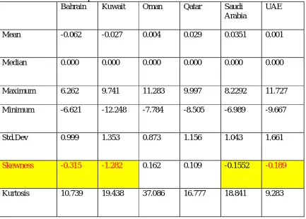
Table 1: The descriptive statistics of the returns:
Bahrain Kuwait Oman Qatar Saudi
Arabia
UAE
Mean -0.062 -0.027 0.004 0.029 0.0351 0.001
Median 0.000 0.000 0.000 0.000 0.000 0.000
Maximum 6.262 9.741 11.283 9.997 8.2292 11.727
Minimum -6.621 -12.248 -7.784 -8.505 -6.989 -9.667
Std.Dev 0.999 1.353 0.873 1.156 1.043 1.661
Skewness -0.315 -1.282 0.162 0.109 -0.1552 -0.189
25
Jarque-Bera test 4066.974* 18671.57* 78480.59* 12822.94* 16693.09* 2681.160*
*Significance at 1% level.
The descriptive statistics portrayed above provide a bird’s eye view on returns of the series. From table 1 it is clearly evident that returns of Bahrain, Kuwait, Saudi Arabia and UAE are negatively skewed which indicates that negative stock returns are more common than positive returns. In other words it is that, there is a greater probability of large decrease in returns than increase. The kurtosis of all the series depicts that the returns have fatter tail and higher peaks. The low mean and variance shows low expected returns and risk. UAE index show a higher standard deviation or risk in the security when compared to other indices followed by Kuwait index. The Jarque Bera statistics rejects the null hypothesis of normality of the returns and thus all the series are identified with returns not normally distributed.
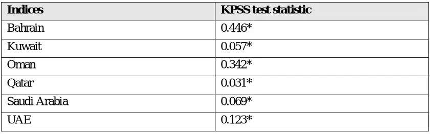
Any time series data needs assurance of the stationarity i.e. there shouldn’t be any unit root issues in the series. But there are evidences where time series data show a non stationarity (Engle & Granger 1987). Hence before going into in-depth modelling of the data it is necessary to check the stationarity property of the series. In order to check stationarity or otherwise KPSS test 8 has been used, which was introduced by Kwiatkowski et al (1992) here. It assumes that the null hypothesis of the series is stationary.
Table 2: The Unit root results of the returns.
Indices KPSS test statistic
Bahrain 0.446*
Kuwait 0.057*
Oman 0.342*
Qatar 0.031*
Saudi Arabia 0.069*
UAE 0.123*
The unit root results from KPSS test shows that all the series are stationary which accepts the null hypothesis since the H0 of KPSS is the series are stationary.
Like stationarity issue in a time series data, there exist a requirement prior to volatility modelling that the residuals of the series should be homoscedastic and there shouldn’t be any ARCH effect9 in the series.
In order to check the homoscedasticity of residuals the serial correlation test10 was conducted and results showed that there was serial correlation within the residuals of all the
8
KPSS Test: The alternative unit root test introduced by Kwiatkowski – Phillips – Schmit – Shin (1992) has
the null hypothesis stationarity of a series around either mean or a linear trend.The model takes the following
form :
1
t t t
t t t
y t r
r r
9
26
series up to 32th lag. After the test of serial correlation ARCH LM test was conducted to identify the ARCH effect. It is calculated by regressing squared residuals on a constant at P lags.
Table 3: Results of ARCH LM Test.
Bahrain Kuwait Oman Qatar Saudi Arabia UAE
F -statistics 20.535 50.02736 100.68309 182.772 182.953 81.716
Observed R2 20.773* 48.585* 94.902* 164.425* 164.571* 77.890*
*significance at 1% level.
From the table it can be inferred that there was an ARCH effect and null hypothesis of no ARCH effect cannot be accepted. Since the F statistics and observed R2 are significant at 1%, it can be interpreted that there is a further scope for modelling volatility with different ARCH-GARCH models and their extensions. Before attempting the modelling of the volatility the persistence of returns or the volatility clustering if any was traced out. The graph of which is given in annexure. Volatility clustering11 implies a strong correlation in squared returns. In order to test volatility clustering Ljung Box was employed where n as sample size and k as lag length.
Modelling of ARCH & GARCH
With the results of volatility clustering and autocorrelation in residuals, the next step was the need to specify and model the conditional volatility in the market. To fit the best model, Akaike Schwartz Criterion and Schwartz Bayesian Criterion were employed. In order to trace out the persistence in return, volatility clustering is checked at the introduction stage. The modelling of the returns of all the series were done through extensions of ARCH model and then with different variant forms such as Threshold GARCH (T-GARCH) and Exponential GARCH (E-GARCH). The persistence of autoregressiveness was tested through GARCH (1, 1) model where volatility clustering was identified and depicted in graph (1), (2), (3),(4), (5) & (6)12 which clearly indicated that these all these indices followed volatility clustering during periods of turbulence where their prices showed wide swings and periods of tranquillity the wide swings were absent. In the attempt to find out the patterns in modelling and Heteroscedasticity in the residuals the ARCH LM test was employed and it was found that there was no homoscedasticity in the returns which gave further scope for modelling of ARCH models and its variants. Thus GARCH (1, 1) model was fitted to the daily return series.
The specification of GARCH (1, 1) model is as follows;
2 2 2
1 1 1 1 1
t t
--- (2)where t2 conditional variance whereas ω is constant,
α
1ε
2t-1 is Arch termand
β
1
2t-1 is sum of squared residual/ Garch term.The results are presented in table 4 for all the indices. Table 4: Results of GARCH (1, 1).
Indices ω( Constant) α (ARCH term) β (GARCH term) α+β
Bahrain 0.019 0.088* 0.899* 0.811
Kuwait 0.012 0.077* 0.922* 0.999
Oman 0.005 0.146* 0.882* 1.028
10
Serial Correlation Test:In statistics, autocorrelation is a random process which describes the correlation between values of the process at different times, as a function of the two or of the time difference.
11
Volatility clustering simply means that periods of highs will be followed by periods of highs and periods of lows/tranquillity will be followed by periods of lows.
12
27
Qatar 0.002 0.026* 0.969* 0.995
Saudi Arabia 0.019 0.052* 0.925* 0.977
UAE 0.039 0.067* 0.925* 0.989
*Significant at 1 % level
The results of GARCH (1, 1) of the returns of six indices of GCC showed that all the parameters in the GARCH (1, 1) were highly significant at 1% significance level. The highly significance of α (ARCH term) and β (GARCH term) implied that past volatility highly influenced the current volatility of all the series under study. As both α and β were significant, it revealed that the lagged conditional variance and lagged squared variance had impact on current volatility.
From the sum values of co-efficient of α+β of the series it was clearly evident that all the indices showed a value which is close to unity and for Oman it crossed the value of unity. It implies that the volatility of all the series except for Oman was highly persistent with 1% significance level of acceptance.
After processing GARCH (1, 1) model other higher order model13 were employed to check the significance. Higher order GARCH models either did not converge or the parameters were insignificant at the conventional levels of significance. Hence it was concluded that this model perfectly fitted in the process and is a representative of the conditional volatility process of the daily returns of the series. Further diagnostic checking14 of the model also revealed that GARCH (1, 1) was a better fit than highest order ARCH models available.
Asymmetrical response to arrival of news
Since the GARCH (1, 1) model is a symmetric one, there was a need to explore asymmetric models because former model depends only on the magnitude and not on the signs of the returns of the series. On the basis of the results of the volatility ARCH/GARCH model, the symmetry effect or leverage effect can be captured through extensions of GARCH family. Some popular extensions are T-GARCH and E-GARCH, Asymmetric Power GARCH etc. and among them T-GARCH and E-GARCH are most popularly used, as they provide reliable results on asymmetric effect of any series.
The T-GARCH model
As GARCH model generates only symmetric response function, there was a need for a new model which incorporates the asymmetric effect of the shock in a series. Zakoian (1990) and Glosten et al (1993) independently developed the T-GARCH model. The specification for the conditional variance is as follows;
2 2 2 2
1 1 1 1 1 1 1
t t
d
t t
--- (3)where
ϒ
is the coefficient of the leverage term, d
t-1 is the dummy variable and εt-1 =1 when εt-1 <0 & εt-1 =0 when εt-1≥0 . In this model good news (εt-1 <0) and bad news (εt-1>) isexplained as good news has an impact on α and bad effects α+ϒ. If ϒ >0 then there is
leverage effect and ϒ≠ o then the news impact is symmetric.
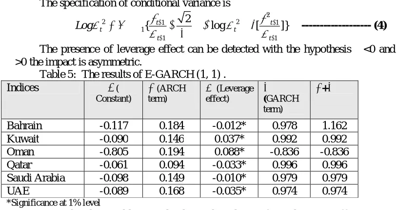
Table 5: The results of T-GARCH (1, 1) .
Indices ω(
Constant)
α (ARCH term)
ϒ (Leverage
effect)
β (GARCH term)
α+β [α+ β+
(ϒ /2)]
13
GARCH (2, 1) was employed and it rejects the homoscedasticity and ARCH test along with Normality test in diagnostic checking.
14
28
Bahrain 0.019 0.091 0.006
(0.5019)
0.899 0.990 0.987
Kuwait 0.0117 0.057 0.0383
(0.000)
0.921 0.978 0.997
Oman 0.005 0.133 0.022
(0.1057)
0.883 1.804 0.988
Qatar 0.003 0.019 0.0382
(0.000)
0.958 0.977 0.996
Saudi Arabia 0.0229 0.0101 0.136
(0.000)
0.902 0.912 0.980
UAE 0.0393 0.045 0.038
(0.0001)
0.925 0.970 1.433
Table 5 presents the asymmetric effect of daily returns of six indices from 2008-2013. It can be noted that the ϒ (Leverage effect) coefficients of all the series were positive and significant except for Bahrain and Oman. In case of Bahrain and Oman it showed a positive sign with an insignificant P value which implies that there was no asymmetry or leverage effect. The coefficients of Kuwait, Qatar, Saudi Arabia and UAE implied that there was a asymmetry effect which indicate that positive shocks had large effect on next period volatility than negative shocks.
The E-GARCH model
The E-GARCH or exponential GARCH was developed by Nelson (1991). Since T-GARCH restricts the sign of variance to positive; E-T-GARCH uses the logarithm of t2 which makes the conditional variance regardless of the signs of co-efficient in the results.
The specification of conditional variance is
2
2 1 2 1
1
1 1
2
{ t log [ t ]}
t t
t t
Log
--- (4)
The presence of leverage effect can be detected with the hypothesis ϒ<0 and if its
ϒ>0 the impact is asymmetric.
Table 5: The results of E-GARCH (1, 1) .
Indices ω(
Constant)
α (ARCH term)
ϒ(Leverage effect)
β (GARCH term)
α+β
Bahrain -0.117 0.184 -0.012* 0.978 1.162
Kuwait -0.090 0.146 0.037* 0.992 0.992
Oman -0.805 0.194 0.088* -0.836 -0.836
Qatar -0.061 0.094 -0.033* 0.996 0.996
Saudi Arabia -0.098 0.149 -0.010* 0.979 0.979
UAE -0.089 0.168 -0.035* 0.974 0.974
*Significance at 1% level
co-29
efficient which implies that positive shocks impacted more on the conditional volatility than negative shocks.
Concluding Remarks
In this paper, attempts have been made to examine the asymmetric conditional volatility of Shariah index of GCC countries with the daily returns ranging a period of 5 years from 01/12/2008 to 31/08/2013. From the descriptive statistics it was clearly evident that UAE was the riskiest index among all the other indices as its standard deviation was highest. Then the attempt was made to model the volatility with GARCH models after detecting the serial correlation and ARCH effect in the series.
The conditional volatility was measured through GARCH (1, 1) model and its extensions. It was noted from the results of GARCH (1, 1) that all the parameters in the GARCH (1, 1) are highly significant at 1% significance level. The highly significant α (ARCH term) and β (GARCH term) implied that past volatility highly influenced the current volatility of all the series under study. The asymmetrical GARCH models outperformed the symmetrical GARCH models. On application of E-GARCH (1, 1) and T-GARCH (1, 1) it was found that there was leverage effect in the all the indices with few exceptions. The leverage terms of all the series were positive and significant except for Bahrain and Oman. In the case of Bahrain and Oman it showed a positive sign with an insignificant P value which implied that there was no asymmetry or leverage effect. The coefficients of Kuwait, Qatar, Saudi Arabia and UAE indicated that there was an asymmetry effect, which indicates that positive shocks have large effect on next period volatility than negative shocks. With regard to E-GARCH (1, 1)Bahrain, Qatar, Saudi Arabia and UAE were significant at 1% level with negative coefficient value. This indicates that negative news impacts more on the volatility than positive news/shocks. Kuwait and Oman shows high significance at 1% level with positive co-efficient indicating higher impact of positive shocks impact more on the conditional volatility.
The implication of the study for the investor is that the asymmetric GARCH models of the series can be used by investors to forecast future volatility of the market. Also further studies can be made on the time varying nature and month effect of the indices which can help the investors to take advantage of less risky months and lesser volatility periods.
References I. Journals
1. Akgiray, V. (1989). “Conditional Heterosckedasticity in time series of stock returns: Evidence and Forecast”. Journal of Business, 62(1), 55-80.
2. Andersen, T.G. and Bollerslev, T. (1996). “Heterogeneous Information Arrivals and Return Volatility Dynamics: Uncovering the Long run in High Frequency Returns”, working paper 5752, National Bureau of Economic Research, MA: Cambridge. 3. Bollerslev, T. (1986). “Generalized Autoregressive Conditional Heteroscedasticity”.
Journal of Econometrics, 31(3), 307-327.
4. Brailsford, Timothy. J. Faff and Robert. W. (1996). “An Evaluation of Volatility Forecasting Techniques”, Journal of Banking and Finance, 20(3), 419-438.
5. Cohrah, A. and Rad, T. (1994). “Statistical properties of Daily returns: Evidence from European Markets”. Journal of Business Finance and Accounting, 21(2), 271-282. 6. Engle, R. F. (1982). “Autoregressive Conditional Heteroscedasticity with estimates of
the variance of United Kingdom inflation”. Econometrica, 50(4), 987-1007.
7. Engle, R. F. and Granger, C. W. J. (1987). “Co-integration and Error-correction: Representation, Estimation and Testing”, Econometrica, 55(2), 251-276.
30
9. Glosten, L.R., Jagannathan, R., Runkle, D., (1993). “On the relation between the expected value and the volatility of the nominal excess return on stocks”. Journal of Finance, 48, 1779–1801.
10. Kwiatkowski, D., Phillips, P.C.B., Schmidt, P., and Shin, Y. (1992). “Testing the Null Hypothesis of Stationarity against the Alternative of a Unit Root”. Journal of Econometrics, 54, 159–178.
11. Nelson, D. B. (1991). “Conditional Heterosckedasticity in Asset returns: A New Approach”, Econometrica, 59(2), 347-375.
12. Pagan. A.R. and Schwert, G.W. (1990). “Alternative models for Conditional Models for conditional stock volatility”, Journal of Econometrics, 45(1-2), 267-290.
13. Pandey. A. (2005). “Volatility models and their Performance in Indian Capital Market”, Vikalpa, 30(2), 27-46.
14. Romli, N., Mohammad, A.Z.S., & Yusuf, M.F.M. (2012). “Volatility analysis of FTSE Bursa Malaysia: A study of the problems of Islamic stock market speculation in the period 2007-2010”. African Journal of Business Management, 6(29), 8490-8495. 15. Shumi. A. Akhtar., Jahromi. M., John. K. and Moise. C. E. (2011). “Intensity of
volatility linkage between Islamic and Conventional markets”. Working Paper Chicago meeting papers, AFA 2012, 49 pages.
16. Tse, Y.K., & Tung, K.H. (1992). “Forecasting volatility in the Singapore stock market”. Asia Pacific Journal of Management, 9, 1-13.
17. Zakoian, J. M. (1990). “Threshold Heterosckedasticity models”, Paris: CREST, INSEE.
18. Zakoian, J.M. (1994). “Threshold Heterosckedasticity models”, Journal of Economic Dynamics, 18(5), 931-955.
II. Books
1. Brooks, C. (2002), Introductory Econometrics for Finance, Cambridge University Press, London.
2. McIver, J. (2001), Microeconomics, The McGraw-Hill, Sydney.
31 Annexure
Graph showing Volatility Clustering of Indices
-10 -5 0 5 10 15 -10 -5 0 5 10 15
IV I II III IV I II III IV I II III IV I II III IV I II III 2009 2010 2011 2012 2013
Residual Actual Fitted
-15 -10 -5 0 5 10 -15 -10 -5 0 5 10
IV I II III IV I II III IV I II III IV I II III IV I II III
2009 2010 2011 2012 2013
Residual Actual Fitted
-8 -4 0 4 8 12 -8 -4 0 4 8 12
IV I II III IV I II III IV I II III IV I II III IV I II III
2009 2010 2011 2012 2013
Residual Actual Fitted
-10 -5 0 5 10 15 -10 -5 0 5 10 15
IV I II III IV I II III IV I II III IV I II III IV I II III
2009 2010 2011 2012 2013
Residual Actual Fitted
-10 -5 0 5 10 15 -10 -5 0 5 10 15
IV I II III IV I II III IV I II III IV I II III IV I II III
2009 2010 2011 2012 2013
Residual Actual Fitted
KUWAIT OMAN
SAUDI ARABIA BAHRAIN