EC2029-Digital-Image-Processing-Lecture-Notes

UNIT-I

DIGITAL IMAGE FUNDAMENTALS AND TRANSFORMS

Elements of visual Perception- Image sampling-quantization- relationship between pixels-Basic geometric transformations- Introduction to Fourier Transform And DFT- Properties of 2D Fourier Transform – FFT-Separable Image Transforms – Walsh- Hadamard – Discrete Cosine Transform, Haar,Slant – Karhunen – Loeve Trans forms.

1. ELEMENTS OF VISUAL PERCEPTION

• The following figure shows the anatomy of the human eye in cross section

• There are two types of receptors in the retina – The rods are long slender receptors

– The cones are generally shorter and thicker in structure • The rods and cones are not distributed evenly around the retina. • Rods and cones operate differently

– Rods are more sensitive to light than cones.

– At low levels of illumination the rods provide a visual response called scotopic vision

– Cones respond to higher levels of illumination; their response is called photopic vision

Page 2 of 137

• There are three basic types of cones in the retina

• These cones have different absorption characteristics as a function of wavelength with peak absorptions in the red, green, and blue regions of the optical spectrum. • is blue, b is green, and g is red

Most of the cones are at the fovea. Rods are spread just about everywhere except the fovea

Page 4 of 137 1.3 CONTRAST SENSITIVITY

• The response of the eye to changes in the intensity of illumination is nonlinear • Consider a patch of light of intensity i+dI surrounded by a background intensity I

as shown in the following figure

• Over a wide range of intensities, it is found that the ratio dI/I, called the Weber fraction, is nearly constant at a value of about 0.02.

• This does not hold at very low or very high intensities

• Furthermore, contrast sensitivity is dependent on the intensity of the surround. Consider the second panel of the previous figure.

1.4 LOGARITHMIC RESPONSE OF CONES AND RODS

• To test the hypothesis that the response of the cones and rods are logarithmic, we examine the following two cases:

• If the intensity response of the receptors to intensity is linear, then the derivative of the response with respect to intensity should be a constant. This is not the case as seen in the next figure.

• To show that the response to intensity is logarithmic, we take the logarithm of the intensity response and then take the derivative with respect to intensity. This derivative is nearly a constant proving that intensity response of cones and rods can be modeled as a logarithmic response.

• Another way to see this is the following, note that the differential of the logarithm of intensity is d(log(I)) = dI/I. Figure 2.3-1 shows the plot of dI/I for the intensity response of the human visual system.

Page 6 of 137 1.5 SIMULTANEOUS CONTRAST

• The simultaneous contrast phenomenon is illustrated below. • The small squares in each image are the same intensity.

• Because the different background intensities, the small squares do not appear equally bright.

• Perceiving the two squares on different backgrounds as different, even though they are in fact identical, is called the simultaneous contrast effect.

• Psychophysically, we say this effect is caused by the difference in the backgrounds, but what is the physiological mechanism behind this effect?

1.6 LATERAL INHIBITION

• Record signal from nerve fiber of receptor A.

• Illumination of receptor A alone causes a large response.

• Add illumination to three nearby receptors at B causes the response at A to decrease.

• Increasing the illumination of B further decreases A‘s response.

• Thus, illumination of the neighboring receptors inhibited the firing of receptor A. • This inhibition is called lateral inhibition because it is transmitted laterally, across

the retina, in a structure called the lateral plexus.

• A neural signal is assumed to be generated by a weighted contribution of many spatially adjacent rods and cones.

• Some receptors exert an inhibitory influence on the neural response.

• The weighting values are, in effect, the impulse response of the human visual system beyond the retina.

• Another effect that can be explained by the lateral inhibition. • The Mach band effect is illustrated in the figure below. • The intensity is uniform over the width of each bar.

• However, the visual appearance is that each strip is darker at its right side than its left.

1.8 MACH BAND

• The Mach band effect is illustrated in the figure below.

• A bright bar appears at position B and a dark bar appears at D.

Page 8 of 137

• An observer is shown two sine wave grating transparencies, a reference grating of constant contrast and spatial frequency, and a variable-contrast test grating whose spatial frequency is set at some value different from that of the reference.

• Contrast is defined as the ratio

(max-min)/(max+min)

where max and min are the maximum and minimum of the grating intensity, respectively.

• The contrast of the test grating is varied until the brightness of the bright and dark regions of the two transparencies appear identical.

• In this manner it is possible to develop a plot of the MTF of the human visual system.

• Note that the response is nearly linear for an exponential sine wave grating.

1.10 MONOCHROME VISION MODEL

• The logarithmic/linear system eye model provides a reasonable prediction of visual response over a wide range of intensities.

• However, at high spatial frequencies and at very low or very high intensities, observed responses depart from responses predicted by the model.

• Light exhibits some properties that make it appear to consist of particles; at other times, it behaves like a wave.

• Light is electromagnetic energy that radiates from a source of energy (or a source of light) in the form of waves

• Visible light is in the 400 nm – 700 nm range of electromagnetic spectrum

1.11.1 INTENSITY OF LIGHT

• The strength of the radiation from a light source is measured using the unit called the candela, or candle power. The total energy from the light source, including heat and all electromagnetic radiation, is called radiance and is usually expressed in watts.

• Luminance is a measure of the light strength that is actually perceived by the human eye. Radiance is a measure of the total output of the source; luminance measures just the portion that is perceived.

Brightness is a subjective, psychological measure of perceived intensity.

Brightness is practically impossible to measure objectively. It is relative. For example, a burning candle in a darkened room will appear bright to the viewer; it will not appear bright in full sunshine.

• The strength of light diminishes in inverse square proportion to its distance from its source. This effect accounts for the need for high intensity projectors for showing multimedia productions on a screen to an audience. Human light perception is sensitive but not linear

2. SAMPLING

Page 10 of 137 2.1 1-D: Sounds

Sampling is, for one-dimensional signals, the operation that transforms a continuous-time signal (such as, for instance, the air pressure fluctuation at the entrance of the ear canal) into a time signal, that is a sequence of numbers. The discrete-time signal gives the values of the continuous-discrete-time signal read at intervals of T seconds. The reciprocal of the sampling interval is called sampling rateFs= 1/T

. In this module we do not explain the theory of sampling, but we rather describe its manifestations. For a a more extensive yet accessible treatment, we point to the

Introduction to Sound Processing. For our purposes, the process of sampling a 1-D signal can be reduced to three facts and a theorem.

 Fact 1: The Fourier Transform of a discrete-time signal is a function (called

spectrum) of the continuous variable ω, and it is periodic with period 2π. Given a value of ω, the Fourier transform gives back a complex number that can be interpreted as magnitude and phase (translation in time) of the sinusoidal component at that frequency.

 Fact 2: Sampling the continuous-time signal x(t) with interval T we get the discrete-time signal x(n) =x(nT) , which is a function of the discrete variable n.

 Fact 3: Sampling a continuous-time signal with sampling rate Fs produces a

discrete-time signal whose frequency spectrum is the periodic replication of the original signal, and the replication period is Fs. The Fourier variable ω for functions of discrete variable is converted into the frequency variable f (in Hertz) by means of

 f=

The Figure 1 shows an example of frequency spectrum of a signal sampled with sampling rate Fs. In the example, the continuous-time signal had all and only the frequency components between −Fb and Fb. The replicas of the original spectrum are sometimes called images.

Frequency spectrum of a sampled signal

Figure 1

Given the facts, we can have an intuitive understanding of the Sampling Theorem, historically attributed to the scientists Nyquist and Shannon.

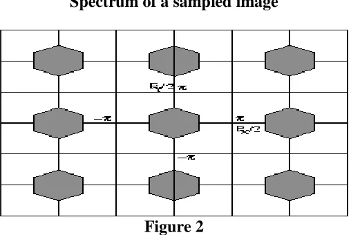
2.2 2-D: Images

Let us assume we have a continuous distribution, on a plane, of values of luminance or, more simply stated, an image. In order to process it using a computer we have to reduce it to a sequence of numbers by means of sampling. There are several ways to sample an image, or read its values of luminance at discrete points. The simplest way is to use a regular grid, with spatial steps X e Y. Similarly to what we did for sounds, we define the spatial sampling rates FX= 1/X

FY= 1/Y

As in the one-dimensional case, also for two-dimensional signals, or images, sampling can be described by three facts and a theorem.

 Fact 1: The Fourier Transform of a discrete-space signal is a function (called

spectrum) of two continuous variables ωX and ωY, and it is periodic in two dimensions with periods 2π. Given a couple of values ωX and ωY, the Fourier transform gives back a complex number that can be interpreted as magnitude and phase (translation in space) of the sinusoidal component at such spatial frequencies.



 Fact 2: Sampling the continuous-space signal s(x,y) with the regular grid of steps

X, Y, gives a discrete-space signal s(m,n) =s(mX,nY) , which is a function of the discrete variables m and n.

Fact 3: Sampling a continuous-space signal with spatial frequencies FX and FY

gives a discrete-space signal whose spectrum is the periodic replication along the grid of steps FX and FY of the original signal spectrum. The Fourier variables ωX and ωY correspond to the frequencies (in cycles per meter) represented by the variables fX= ωX/2πX

 And fy= ωY /2πY

Page 12 of 137

Spectrum of a sampled image

Figure 2

Given the above facts, we can have an intuitive understanding of the Sampling Theorem.

3. QUANTIZATION

With the adjective "digital" we indicate those systems that work on signals that are represented by numbers, with the (finite) precision that computing systems allow. Up to now we have considered discrete-time and discrete-space signals as if they were collections of infinite-precision numbers, or real numbers. Unfortunately, computers only allow to represent finite subsets of rational numbers. This means that our signals are subject to quantization.

For our purposes, the most interesting quantization is the linear one, which is usually occurring in the process of conversion of an analog signal into the digital domain. If the memory word dedicated to storing a number is made of b bits, then the range of such number is discretized into 2b quantization levels. Any value that is found between two quantization levels can be approximated by truncation or rounding to the closest value. The Figure 3 shows an example of quantization with representation on 3 bits in two's complement.

The approximation introduced by quantization manifests itself as a noise, called

quantization noise. Often, for the analysis of sound-processing circuits, such noise is assumed to be white and de-correlated with the signal, but in reality it is perceptually tied to the signal itself, in such an extent that quantization can be perceived as an effect.

To have a visual and intuitive exploration of the phenomenon of quantization, consider the applet that allows to vary between 1 and 8 the number of bits dedicated to the representation of each of the RGB channels representing color. The same number of bits is dedicated to the representation of an audio signal coupled to the image. The visual effect that is obtained by reducing the number of bits is similar to a solarization.

4. BASIC RELATIONSHIP BETWEEN PIXELS

In digital imaging, a pixel (or picture element) is a single point in a raster image. The pixel is the smallest addressable screen element; it is the smallest unit of picture that can be controlled. Each pixel has its own address. The address of a pixel corresponds to its coordinates. Pixels are normally arranged in a 2-dimensional grid, and are often represented using dots or squares. Each pixel is a sample of an original image; more samples typically provide more accurate representations of the original. The intensity of each pixel is variable. In color image systems, a color is typically represented by three or four component intensities such as red, green, and blue, or cyan, magenta, yellow, and black.

The word pixel is based on a contraction of pix ("pictures") and el (for "element"); similar formations with el for "element" include the words: voxel and texel.

4.2 Bits per pixel

The number of distinct colors that can be represented by a pixel depends on the number of bits per pixel (bpp). A 1 bpp image uses 1-bit for each pixel, so each pixel can be either on or off. Each additional bit doubles the number of colors available, so a 2 bpp image can have 4 colors, and a 3 bpp image can have 8 colors:

 1 bpp, 21 = 2 colors (monochrome)

 2 bpp, 22 = 4 colors

 3 bpp, 23 = 8 colors

 8 bpp, 28 = 256 colors

 16 bpp, 216 = 65,536 colors ("Highcolor" )

 24 bpp, 224 ≈ 16.8 million colors ("Truecolor")

Page 14 of 137

more sensitive to errors in green than in the other two primary colors. For applications involving transparency, the 16 bits may be divided into five bits each of red, green, and available: this means that each 24-bit pixel has an extra 8 bits to describe its blue, with one bit left for transparency. A 24-bit depth allows 8 bits per component. On some systems, 32-bit depth is opacity (for purposes of combining with another image).

Selected standard display resolutions include:

Name Megapixels Width x Height

CGA 0.064 320×200

EGA 0.224 640×350

VGA 0.3 640×480

SVGA 0.5 800×600

XGA 0.8 1024×768

SXGA 1.3 1280×1024

UXGA 1.9 1600×1200

WUXGA 2.3 1920×1200

5. BASIC GEOMETRIC TRANSFORMATIONS

Transform theory plays a fundamental role in image processing, as working with the transform of an image instead of the image itself may give us more insight into the properties of the image. Two dimensional transforms are applied to image enhancement, restoration, encoding and description.

5.1. UNITARY TRANSFORMS

For a one dimensional sequence {f(x),0xN1} represented as a vector





N f f f

f  (0) (1) ( 1) of size N, a transformation may be written as

1 0 , ) ( ) , ( ) ( 1 0        

T u x f x u N

u g f T g N x

where g(u) is the transform (or transformation) of f(x), and T(u,x) is the so called forward transformation kernel. Similarly, the inverse transform is the relation

      1 0 1 0 ), ( ) , ( ) ( N u N x u g u x I x f

or written in a matrix form

g T g I

f    1

where I(x,u) is the so called inverse transformation kernel. If

T

the matrix T is called unitary, and the transformation is called unitary as well. It can be proven (how?) that the columns (or rows) of an NN unitary matrix are orthonormal and therefore, form a complete set of basis vectors in the Ndimensional vector space. In that case

    _{  }  1 0 ) ( ) , ( ) ( N u T u g x u T x f g T f

The columns of TT, that is, the vectors Tu 





 

 _

are called the basis vectors of T .

5.1.2 Two dimensional signals (images)

As a one dimensional signal can be represented by an orthonormal set of basis vectors, an image can also be expanded in terms of a discrete set of basis arrays called basis images through a two dimensional (image) transform.

For an NN image f x y( , ) the forward and inverse transforms are given below

      1 0 1 0 ) , ( ) , , , ( ) , ( N x N y y x f y x v u T v u g       1 0 1 0 ) , ( ) , , , ( ) , ( N u N v v u g v u y x I y x f

where, again, T(u,v,x,y) and I(x,y,u,v) are called the forward and inverse transformation kernels, respectively.

The forward kernel is said to be separable if

) , ( ) , ( ) , , ,

(uv x y T₁u xT₂ v y

T 

It is said to be symmetric if T₁ is functionally equal to T₂ such that

) , ( ) , ( ) , , ,

(u v x y T1 u xT1 v y

T 

The same comments are valid for the inverse kernel.

If the kernel T(u,v,x,y) of an image transform is separable and symmetric, then the

transform    

         1 0 1 1 0 1 1 0 1 0 ) , ( ) , ( ) , ( ) , ( ) , , , ( ) , ( N x N y N x N y y x f y v T x u T y x f y x v u T v u

g can be written in

matrix form as follows

T

T f T

g 1  1

where f is the original image of size NN, and T₁ is an NN transformation matrix

with elements tij T1(i,j). If, in addition, T1 is a unitary matrix then the transform is

called separable unitary and the original image is recovered through the relationship 

 _{ }

T1 g T1

f T

5.1.3 Fundamental properties of unitary transforms

5.1.3.1 The property of energy preservation

In the unitary transformation

Page 16 of 137

it is easily proven (try the proof by using the relation T1 TT) that

2 2

f

g 

Thus, a unitary transformation preserves the signal energy. This property is called energy preservation property.

This means that every unitary transformation is simply a rotation of the vector f in the

N- dimensional vector space.

For the 2-D case the energy preservation property is written as

f x y g u v

y N x N v N u N

( , )2 ( , ) 0 1 0 1 ₂ 0 1 0 1             

5.1.3.2The property of energy compaction

Most unitary transforms pack a large fraction of the energy of the image into relatively few of the transform coefficients. This means that relatively few of the transform coefficients have significant values and these are the coefficients that are close to the origin (small index coefficients).

This property is very useful for compression purposes. (Why?)

5.2. THE TWO DIMENSIONAL FOURIER TRANSFORM

The Fourier transform is extended to a function f x y( , ) of two variables. If

f x y( , ) is continuous and integrable and F u v( , ) is integrable, the following Fourier transform pair exists:

      

 f x y e dxdy

v u

F( , ) ( , ) j2(ux vy)

  

 



 F u ve dudv

y x

f j2 (ux vy)

2 ( , )

) 2 ( 1 ) , (  

In general F u v( , ) is a complex-valued function of two real frequency variables u v, and hence, it can be written as:

) , ( ) , ( ) ,

(u v Ru v jI u v

F  

The amplitude spectrum, phase spectrum and power spectrum, respectively, are defined as follows.

F u v( , )  R u v2( , )I2( , )u v

        ) , ( ) , ( tan ) , ( 1 v u R v u I v u 

5.2.2 Discrete space and continuous frequency

For the case of a discrete sequence f(x,y) of infinite duration we can define the 2-D discrete space Fourier transform pair as follows

          x y vy xu j e y x f v u

F( , ) ( , ) ( )

dudv e v u F y x

f j xu vy

u v

) (

2 ( , )

) 2 ( 1 ) , (          

F u v( , ) is again a complex-valued function of two real frequency variables u v,

and it is periodic with a period 22, that is to say F u v( , )F u( 2, )v F u v( , 2)

The Fourier transform of f x y( , ) is said to converge uniformly when F u v( , ) is finite and

) , ( ) , ( lim lim 1 1 2 2 2 1 ) ( v u F e y x f N N x N N y vy xu j N

N _ _{ }    

 

 for all u v, .

When the Fourier transform of f x y( , ) converges uniformly, F u v( , ) is an analytic function and is infinitely differentiable with respect to u and v.

5.2.3 Discrete space and discrete frequency: The two dimensional Discrete Fourier Transform (2-D DFT)

If f x y( , ) is an MN array, such as that obtained by sampling a continuous function of two dimensions at dimensions MandN on a rectangular grid, then its two dimensional Discrete Fourier transform (DFT) is the array given by

        1 0 1 0 ) / / ( 2 ) , ( 1 ) , ( M x N y N vy M ux j e y x f MN v u F  1 , , 0   M

u  , v0,,N1

and the inverse DFT (IDFT) is

f x y F u v ej ux M vy N

v N u M ( , ) ( , ) ( /  / )       2 0 1 0 1 

When images are sampled in a square array, M N and

F u v

N f x y e

j ux vy N y N x N ( , ) ( , )  (  )/       1 2 0 1 0 1 

f x y

N F u v e

j ux vy N v N u N ( , ) ( , ) (  )/       1 2 0 1 0 1 

It is straightforward to prove that the two dimensional Discrete Fourier Transform is separable, symmetric and unitary.

5.2.3.1 Properties of the 2-D DFT

Most of them are straightforward extensions of the properties of the 1-D Fourier Transform. Advise any introductory book on Image Processing.

Completeness

Page 18 of 137

with C denoting the set of complex numbers. In other words, for any N > 0, an N -dimensional complex vector has a DFT and an IDFT which are in turn N-dimensional complex vectors.

Orthogonality

The vectors form an orthogonal basis over the set of N-dimensional complex vectors:

where is the Kronecker delta. This orthogonality condition can be used to derive the formula for the IDFT from the definition of the DFT, and is equivalent to the unitarity property below.

The Plancherel theorem and Parseval's theorem

If Xk and Yk are the DFTs of xn and yn respectively then the Plancherel theorem states:

where the star denotes complex conjugation. Parseval's theorem is a special case of the Plancherel theorem and states:

These theorems are also equivalent to the unitary condition below.

Periodicity

If the expression that defines the DFT is evaluated for all integers k instead of just for , then the resulting infinite sequence is a periodic extension of the DFT, periodic with period N.

Similarly, it can be shown that the IDFT formula leads to a periodic extension.

The shift theorem

Multiplying xn by a linear phase for some integer m corresponds to a

circular shift of the output Xk: Xk is replaced by Xk − m, where the subscript is interpreted modulo N (i.e., periodically). Similarly, a circular shift of the input xn corresponds to multiplying the output Xk by a linear phase. Mathematically, if {xn} represents the vector x then

if

then

and

Circular convolution theorem and cross-correlation theorem

The convolution theorem for the continuous and discrete time Fourier transforms indicates that a convolution of two infinite sequences can be obtained as the inverse transform of the product of the individual transforms. With sequences and transforms of length N, a circularity arises:

The quantity in parentheses is 0 for all values of m except those of the form n − l

Page 20 of 137

which is the convolution of the sequence with a periodically extended sequence defined by:

Similarly, it can be shown that:

which is the cross-correlation of and

A direct evaluation of the convolution or correlation summation (above) requires

O(N2) operations for an output sequence of length N. An indirect method, using transforms, can take advantage of the O(NlogN) efficiency of the fast Fourier transform (FFT) to achieve much better performance. Furthermore, convolutions can be used to efficiently compute DFTs via Rader's FFT algorithm and Bluestein's FFT algorithm.

Methods have also been developed to use circular convolution as part of an efficient process that achieves normal (non-circular) convolution with an or sequence potentially much longer than the practical transform size (N). Two such methods are called overlap-save and overlap-add[1].

Convolution theorem duality

which is the circular convolution of and .

Trigonometric interpolation polynomial

The trigonometric interpolation polynomial

for N even ,

for N odd,

where the coefficients Xk are given by the DFT of xn above, satisfies the interpolation property p(2πn / N) = xn for .

For even N, notice that the Nyquist component is handled specially.

This interpolation is not unique: aliasing implies that one could add N to any of the complex-sinusoid frequencies (e.g. changing e − it to ei(N − 1)t ) without changing the interpolation property, but giving different values in between the xn points. The choice above, however, is typical because it has two useful properties. First, it consists of sinusoids whose frequencies have the smallest possible magnitudes, and therefore

minimizes the mean-square slope of the interpolating function. Second, if the xn are real numbers, then p(t) is real as well.

In contrast, the most obvious trigonometric interpolation polynomial is the one in which the frequencies range from 0 to N − 1 (instead of roughly − N / 2 to + N / 2 as above), similar to the inverse DFT formula. This interpolation does not minimize the slope, and is not generally real-valued for real xn; its use is a common mistake.

The unitary DFT

Page 22 of 137

where

is a primitive Nth root of unity. The inverse transform is then given by the inverse of the above matrix:

With unitary normalization constants , the DFT becomes a unitary transformation, defined by a unitary matrix:

where det() is the determinant function. The determinant is the product of the eigenvalues, which are always or as described below. In a real vector space, a unitary transformation can be thought of as simply a rigid rotation of the coordinate system, and all of the properties of a rigid rotation can be found in the unitary DFT.

The orthogonality of the DFT is now expressed as an orthonormality condition (which arises in many areas of mathematics as described in root of unity):

If is defined as the unitary DFT of the vector then

If we view the DFT as just a coordinate transformation which simply specifies the components of a vector in a new coordinate system, then the above is just the statement that the dot product of two vectors is preserved under a unitary DFT transformation. For the special case , this implies that the length of a vector is preserved as well—this is just Parseval's theorem:

Expressing the inverse DFT in terms of the DFT

A useful property of the DFT is that the inverse DFT can be easily expressed in terms of the (forward) DFT, via several well-known "tricks". (For example, in computations, it is often convenient to only implement a fast Fourier transform corresponding to one transform direction and then to get the other transform direction from the first.)

First, we can compute the inverse DFT by reversing the inputs:

(As usual, the subscripts are interpreted modulo N; thus, for n = 0, we have xN − 0 = x0.)

Second, one can also conjugate the inputs and outputs:

Third, a variant of this conjugation trick, which is sometimes preferable because it requires no modification of the data values, involves swapping real and imaginary parts (which can be done on a computer simply by modifying pointers). Define swap(xn) as xn with its real and imaginary parts swapped—that is, if xn = a + bi then swap(xn) is b + ai. Equivalently, swap(xn) equals . Then

That is, the inverse transform is the same as the forward transform with the real and imaginary parts swapped for both input and output, up to a normalization (Duhamel

et al., 1988).

Page 24 of 137

is clearly its own inverse: . A closely related

involutary transformation (by a factor of (1+i) /√2) is

, since the (1 + i) factors in cancel the 2. For real inputs , the real part of is none other than the discrete Hartley transform, which is also involutary.

Eigenvalues and eigenvectors

The eigenvalues of the DFT matrix are simple and well-known, whereas the eigenvectors are complicated, not unique, and are the subject of ongoing research.

Consider the unitary form defined above for the DFT of length N, where

. This matrix satisfies the equation:

This can be seen from the inverse properties above: operating twice gives the original data in reverse order, so operating four times gives back the original data and is thus the identity matrix. This means that the eigenvalues λ satisfy a characteristic equation:

λ4

= 1.

Therefore, the eigenvalues of are the fourth roots of unity: λ is +1, −1, +i, or −i.

Since there are only four distinct eigenvalues for this matrix, they have some multiplicity. The multiplicity gives the number of linearly independent eigenvectors corresponding to each eigenvalue. (Note that there are N independent eigenvectors; a unitary matrix is never defective.)

The problem of their multiplicity was solved by McClellan and Parks (1972), although it was later shown to have been equivalent to a problem solved by Gauss (Dickinson and Steiglitz, 1982). The multiplicity depends on the value of N modulo 4, and is given by the following table:

size N λ = +1 λ = −1 λ = -i λ = +i

4m m + 1 m m m − 1

4m + 1 m + 1 m m m

4m + 2 m + 1 m + 1 m m

4m + 3 m + 1 m + 1 m + 1 m

No simple analytical formula for general eigenvectors is known. Moreover, the eigenvectors are not unique because any linear combination of eigenvectors for the same eigenvalue is also an eigenvector for that eigenvalue. Various researchers have proposed different choices of eigenvectors, selected to satisfy useful properties like orthogonality and to have "simple" forms (e.g., McClellan and Parks, 1972; Dickinson and Steiglitz, 1982; Grünbaum, 1982; Atakishiyev and Wolf, 1997; Candan et al., 2000; Hanna et al., 2004; Gurevich and Hadani, 2008). However two simple closed-form analytical eigenvectors for special DFT period N were found (Kong, 2008):

For DFT period N = 2L + 1 = 4K +1, where K is an integer, the following is an eigenvector of DFT:

For DFT period N = 2L = 4K, where K is an integer, the following is an eigenvector of DFT:

The choice of eigenvectors of the DFT matrix has become important in recent years in order to define a discrete analogue of the fractional Fourier transform—the DFT matrix can be taken to fractional powers by exponentiating the eigenvalues (e.g., Rubio and Santhanam, 2005). For the continuous Fourier transform, the natural orthogonal eigenfunctions are the Hermite functions, so various discrete analogues of these have been employed as the eigenvectors of the DFT, such as the Kravchuk polynomials (Atakishiyev and Wolf, 1997). The "best" choice of eigenvectors to define a fractional discrete Fourier transform remains an open question, however.

The real-input DFT

If are real numbers, as they often are in practical applications, then the DFT obeys the symmetry:

The star denotes complex conjugation. The subscripts are interpreted modulo N.

Page 26 of 137

real, so there are exactly N non-redundant real numbers in the first half + Nyquist element of the complex output X.

Using Euler's formula, the interpolating trigonometric polynomial can then be interpreted as a sum of sine and cosine functions.

5.2.3.2 The importance of the phase in 2-D DFT. Image reconstruction from amplitude or phase only.

The Fourier transform of a sequence is, in general, complex-valued, and the unique representation of a sequence in the Fourier transform domain requires both the phase and the magnitude of the Fourier transform. In various contexts it is often desirable to reconstruct a signal from only partial domain information. Consider a 2-D sequence

) , (x y

f with Fourier transform F(u,v)





) , ( ) , ( } , ( { ) ,

( j f uv

e v u F y x f v u

F   

It has been observed that a straightforward signal synthesis from the Fourier transform phase f(u,v) alone, often captures most of the intelligibility of the original

image f(x,y) (why?). A straightforward synthesis from the Fourier transform magnitude

) , (u v

F alone, however, does not generally capture the original signal‘s intelligibility.

The above observation is valid for a large number of signals (or images). To illustrate this, we can synthesise the phase-only signal f_p(x,y) and the magnitude-only signal

) , (x y

f_m by





1 ) ,

( j uv

p

f

e y

x

f  





1 ) , ( ) , ( j

m x y F u v e

f 

and observe the two results (Try this exercise in MATLAB).

An experiment which more dramatically illustrates the observation that phase-only signal synthesis captures more of the signal intelligibility than magnitude-only synthesis, can be performed as follows.

Consider two images f(x,y) and g(x,y). From these two images, we synthesise two other images f₁(x,y) and g₁(x,y) by mixing the amplitudes and phases of the original images as follows:





1( , ) ( , )

v u j f e v u G y x

f  





1( , ) ( , )

v u j g e v u F y x

g  

5.3 FAST FOURIER TRANSFORM (FFT)

In this section we present several methods for computing the DFT efficiently. In view of the importance of the DFT in various digital signal processing applications, such as linear filtering, correlation analysis, and spectrum analysis, its efficient computation is a topic that has received considerable attention by many mathematicians, engineers, and applied scientists.

From this point, we change the notation that X(k), instead of y(k) in previous sections, represents the Fourier coefficients of x(n).

Basically, the computational problem for the DFT is to compute the sequence {X(k)} of N complex-valued numbers given another sequence of data {x(n)} of length N, according to the formula

In general, the data sequence x(n) is also assumed to be complex valued. Similarly, The IDFT becomes

Since DFT and IDFT involve basically the same type of computations, our discussion of efficient computational algorithms for the DFT applies as well to the efficient computation of the IDFT.

We observe that for each value of k, direct computation of X(k) involves N

complex multiplications (4N real multiplications) and N-1 complex additions (4N-2 real additions). Consequently, to compute all N values of the DFT requires N 2 complex multiplications and N 2-N complex additions.

Direct computation of the DFT is basically inefficient primarily because it does not exploit the symmetry and periodicity properties of the phase factor WN. In particular,

these two properties are :

Page 28 of 137

6. SEPARABLE IMAGE TRANSFORMS

6.1

THE DISCRETE COSINE TRANSFORM (DCT)

6.1.1 One dimensional signals

This is a transform that is similar to the Fourier transform in the sense that the new independent variable represents again frequency. The DCT is defined below.

        1 0 2 ) 1 2 ( cos ) ( ) ( ) ( N x N u x x f u a u

C  , u0,1,,N1

with a(u) a parameter that is defined below.

         1 , , 1 / 2 0 / 1 ) ( N u N u N u a 

The inverse DCT (IDCT) is defined below.

        1 0 2 ) 1 2 ( cos ) ( ) ( ) ( N u N u x u C u a x f 

6.1.2 Two dimensional signals (images) For 2-D signals it is defined as

                N v y N u x y x f v a u a v u C N x N y 2 ) 1 2 ( cos 2 ) 1 2 ( cos ) , ( ) ( ) ( ) , ( 1 0 1 0                   N v y N u x v u C v a u a y x f N u N v 2 ) 1 2 ( cos 2 ) 1 2 ( cos ) , ( ) ( ) ( ) , ( 1 0 1 0   ) (u

a is defined as above and u,v0,1,,N1

6.1.3 Properties of the DCT transform

 The DCT is a real transform. This property makes it attractive in comparison to the Fourier transform.

 The DCT has excellent energy compaction properties. For that reason it is widely used in image compression standards (as for example JPEG standards).

 There are fast algorithms to compute the DCT, similar to the FFT for computing the DFT.

6.2

WALSH TRANSFORM (WT)

6.2.1 One dimensional signals

This transform is slightly different from the transforms you have met so far. Suppose we have a function f(x),x0,,N1 where N2n and its Walsh transform W(u).

If we use binary representation for the values of the independent variables x and u we need n





10 ( ) ( ) ( )

)

(x  bn xbn x b x , (u)10





Example

If f(x),x0,,7,(8samples) then n3 and for x6, 0 ) 6 ( , 1 ) 6 ( , 1 ) 6 ( (110) =

6 2b2  b1  b0 

We define now the 1-D Walsh transform as

         _

 1 

0 1 0 ) ( ) ( 1 ) 1 ( ) ( 1 ) ( N x n i u b x bi n i

x f N u

W or

         1 0 ) ( ) ( ₁ 1 0 ) 1 )( ( 1 ) ( N x u b x b _{n i}

n i i x f N u W

The array formed by the Walsh kernels is again a symmetric matrix having orthogonal rows and columns. Therefore, the Walsh transform is and its elements are of the form

      1 0 ) ( ) ( ₁ ) 1 ( ) , ( n i u b x b_{i n i}

x u

T . You can immediately observe that T(u,x)0 or 1 depending on the

values of b_i(x) and b_n1i(u). If the Walsh transform is written in a matrix form

f T

W  

the rows of the matrix T which are the vectors







 



10 ( ) ( ) ( ) 00 0

)

(u  b_n u b_n u b u   and hence, b_n1i(u)0, for any i. Thus, T(0,x)1

and 

  1 0 ) ( 1 ) 0 ( N x x f N

W . We see that the first element of the Walsh transform in the mean of the

original function f(x) (the DC value) as it is the case with the Fourier transform.

The inverse Walsh transform is defined as follows.

         _

 1 

0 1 0 ) ( ) ( 1 ) 1 ( ) ( ) ( N u n i u b x bi n i

u W x

f or

         1 0 ) ( ) ( ₁ 1 0 ) 1 )( ( ) ( N u u b x b _{n i}

n i i u W x f

6.2.2 Two dimensional signals

The Walsh transform is defined as follows for two dimensional signals.

             _

 1  

0 1 0 )) ( ) ( ) ( ) ( ( 1 0 1 1 ) 1 ( ) , ( 1 ) , ( N x n i v b y b u b x b N y i n i i n i y x f N v u

W or

Page 30 of 137

The inverse Walsh transform is defined as follows for two dimensional signals.

             _

 1  

0 1 0 )) ( ) ( ) ( ) ( ( 1 0 1 1 ) 1 ( ) , ( 1 ) , ( N u n i v b y b u b x b N v i n i i n i v u W N y x

f or

               1 0 )) ( ) ( ) ( ) ( ( 1 0 1 1 1 0 ) 1 ( ) , ( 1 ) , ( N u v b y b u b x b N v i n i i n i n i v u W N y x f

6.2.3 Properties of the Walsh Transform

 Unlike the Fourier transform, which is based on trigonometric terms, the Walsh transform consists of a series expansion of basis functions whose values are only 1 or 1 and they have the form of square waves. These functions can be implemented more efficiently in a digital environment than the exponential basis functions of the Fourier transform.

 The forward and inverse Walsh kernels are identical except for a constant multiplicative

factor of

N

1

for 1-D signals.

 The forward and inverse Walsh kernels are identical for 2-D signals. This is because the array formed by the kernels is a symmetric matrix having orthogonal rows and columns, so its inverse array is the same as the array itself.

 The concept of frequency exists also in Walsh transform basis functions. We can think of frequency as the number of zero crossings or the number of transitions in a basis vector and we call this number sequency. The Walsh transform exhibits the property of energy compaction as all the transforms that we are currently studying. (why?)

 For the fast computation of the Walsh transform there exists an algorithm called Fast Walsh Transform (FWT). This is a straightforward modification of the FFT. Advise any introductory book for your own interest.

6.3

HADAMARD TRANSFORM (HT)

6.3.1 Definition

In a similar form as the Walsh transform, the 2-D Hadamard transform is defined as follows.

Forward              _  1 0 1 0 )) ( ) ( ) ( ) ( ( 1 0 ) 1 ( ) , ( 1 ) , ( N x n i v b y b u b x b N y i i i i y x f N v u

H , N2nor

          1 0 )) ( ) ( ) ( ) ( ( 1 0 1 0 ) 1 )( , ( 1 ) , ( N x v b y b u b x b N y i i i i n i y x f N v u H Inverse              _  1 0 1 0 )) ( ) ( ) ( ) ( ( 1 0 ) 1 ( ) , ( 1 ) , ( N u n i v b y b u b x b N v i i i i v u H N y x

f etc.

6.3.2 Properties of the Hadamard Transform

 The Hadamard transform differs from the Walsh transform only in the order of basis functions. The order of basis functions of the Hadamard transform does not allow the fast computation of it by using a straightforward modification of the FFT. An extended version of the Hadamard transform is the Ordered Hadamard Transform for which a fast algorithm called Fast Hadamard Transform (FHT) can be applied.

 An important property of Hadamard transform is that, letting H_N represent the matrix of order N, the recursive relationship is given by the expression

   

 

 

N N

N N N

H H

H H H2

6.4

KARHUNEN-LOEVE (KLT) or HOTELLING TRANSFORM

The Karhunen-Loeve Transform or KLT was originally introduced as a series expansion for continuous random processes by Karhunen and Loeve. For discrete signals Hotelling first studied what was called a method of principal components, which is the discrete equivalent of the KL series expansion. Consequently, the KL transform is also called the Hotelling transform or the method of principal components. The term KLT is the most widely used.

6.4.1 The case of many realisations of a signal or image (Gonzalez/Woods)

The concepts of eigenvalue and eigevector are necessary to understand the KL transform.

If C is a matrix of dimension nn, then a scalar  is called an eigenvalue of C if there is a

nonzero vector e in Rn such that

e e

C 

The vector e is called an eigenvector of the matrix C corresponding to the eigenvalue .

(If you have difficulties with the above concepts consult any elementary linear algebra book.)

Consider a population of random vectors of the form

   

 

   

 



n

x x x

x 

2 1

The mean vector of the population is defined as

 

The operator E refers to the expected value of the population calculated theoretically using the probability density functions (pdf) of the elements x_i and the joint probability density functions between the elements xi and xj.

The covariance matrix of the population is defined as





x x

x E x m x m

Page 32 of 137

Because x is n-dimensional, C_x and (xmx)(xmx)T are matrices of order nn. The element cii of Cx is the variance of xi, and the element cij of Cx is the covariance between the elements xi and xj. If the elements xi and xj are uncorrelated, their covariance is zero and, therefore, cij cji 0.

For M vectors from a random population, where M is large enough, the mean vector and covariance matrix can be approximately calculated from the vectors by using the following relationships where all the expected values are approximated by summations

   M k k x x M m 1 1 T x x T k M k k

x x x m m

M

C   

1 1

Very easily it can be seen that C_x is real and symmetric. In that case a set of n orthonormal (at this point you are familiar with that term) eigenvectors always exists. Let e_i and _i,

n

i1,2,, , be this set of eigenvectors and corresponding eigenvalues of C_x, arranged in descending order so that _i _i1 for i1,2,,n1. Let A be a matrix whose rows are formed from the eigenvectors of C_x, ordered so that the first row of A is the eigenvector corresponding to the largest eigenvalue, and the last row the eigenvector corresponding to the smallest eigenvalue.

Suppose that A is a transformation matrix that maps the vectors x's into vectors y's by using the following transformation

) (x m_x A

y 

The above transform is called the Karhunen-Loeve or Hotelling transform. The mean of the y

vectors resulting from the above transformation is zero (try to prove that) 0

 y

m

the covariance matrix is (try to prove that)

T x y AC A

C 

and C_y is a diagonal matrix whose elements along the main diagonal are the eigenvalues of C_x

(try to prove that)

             n y C    0 0 2 1 

The off-diagonal elements of the covariance matrix are 0 , so the elements of the y

vectors are uncorrelated.

Lets try to reconstruct any of the original vectors x from its corresponding y. Because the rows

of A are orthonormal vectors (why?), then A1 AT, and any vector x can by recovered from its corresponding vector y by using the relation

x T

m y A

Suppose that instead of using all the eigenvectors of C_x we form matrix A_K from the K

eigenvectors corresponding to the K largest eigenvalues, yielding a transformation matrix of order Kn. The y vectors would then be K dimensional, and the reconstruction of any of the

original vectors would be approximated by the following relationship

x T Ky m

A

xˆ 

The mean square error between the perfect reconstruction x and the approximate reconstruction

xˆ is given by the expression

          n K j j K j j n j j ms e 1 1 1    .

By using A_K instead of A for the KL transform we achieve compression of the available data. 6.4.2 The case of one realisation of a signal or image

The derivation of the KLT for the case of one image realisation assumes that the two dimensional signal (image) is ergodic. This assumption allows us to calculate the statistics of the image using only one realisation. Usually we divide the image into blocks and we apply the KLT in each block. This is reasonable because the 2-D field is likely to be ergodic within a small block since the nature of the signal changes within the whole image. Let‘s suppose that f is a vector obtained by lexicographic ordering of the pixels f(x,y) within a block of size MM (placing the rows of the block sequentially).

The mean vector of the random field inside the block is a scalar that is estimated by the approximate relationship    2 1

2 ( )

1 M k

f f k

M m

and the covariance matrix of the 2-D random field inside the block is C_f where 2

1

2 ( ) ( )

1 2

f M

k

ii f k f k m

M

c   

 and

2 1

2 ( ) ( )

1 2 f M k j i

ij f k f k i j m

M c

c      

 

After knowing how to calculate the matrix C_f, the KLT for the case of a single realisation is the same as described above.

6.4.3 Properties of the Karhunen-Loeve transform

Despite its favourable theoretical properties, the KLT is not used in practice for the following reasons.

 Its basis functions depend on the covariance matrix of the image, and hence they have to recomputed and transmitted for every image.

 Perfect decorrelation is not possible, since images can rarely be modelled as realisations of ergodic fields.

 There are no fast computational algorithms for its implementation.

Page 34 of 137 IMPORTANT TWO MARKS QUESTIONS

1. Define subjective brightness and brightness adaptation?

Subjective brightness means intensity as preserved by the human visual system. Brightness adaptation means the human visual system can operate only from

scotopic to glare limit. It cannot operate over the range simultaneously. It accomplishes this large variation by changes in its overall intensity.

2. Define Weber ratio

The ratio of increment of illumination to background of illumination is called as

weber ratio.(ie) i/i

If the ratio ( i/i) is small, then small percentage of change in intensity is needed (ie) good brightness adaptation.

If the ratio ( i/i) is large , then large percentage of change in intensity is needed (ie) poor brightness adaptation.

3. What is meant by machband effect?

Machband effect means the intensity of the stripes is constant. Therefore it preserves the brightness pattern near the boundaries, these bands are called as machband effect.

4. What is simultaneous contrast?

The region reserved brightness not depend on its intensity but also on its background. All centre square have same intensity. However they appear to the eye to become darker as the background becomes lighter.

5. What is meant by illumination and reflectance?

Illumination is the amount of source light incident on the scene. It is represented as i(x, y).

Reflectance is the amount of light reflected by the object in the scene. It is

represented by r(x, y).

6. Define sampling and quantization

Sampling means digitizing the co-ordinate value (x, y). Quantization means digitizing the amplitude value.

7. Find the number of bits required to store a 256 X 256 image with 32 gray levels? 32 gray levels = 25

= 5 bits

256 * 256 * 5 = 327680 bits.

8. What do you meant by Zooming of digital images?

Zooming may be viewed as over sampling. It involves the creation of new pixel locations and the assignment of gray levels to those new locations.

9. What do you meant by shrinking of digital images?

delete every row and column. To reduce possible aliasing effect, it is a good idea to blue an image slightly before shrinking it.

10. What is geometric transformation?

Transformation is used to alter the co-ordinate description of image. The basic geometric transformations are

1. Image translation 2. Scaling

3. Image rotation

11. What is image translation and scaling?

Image translation means reposition the image from one co-ordinate location to another along straight line path.

Scaling is used to alter the size of the object or image (ie) a co-ordinate system is scaled by a factor.

12. What is the need for transform?

The need for transform is most of the signals or images are time domain signal (ie) signals can be measured with a function of time. This representation is not always best. For most image processing applications anyone of the mathematical transformation are applied to the signal or images to obtain further information from that signal.

16 MARKS QUESTIONS

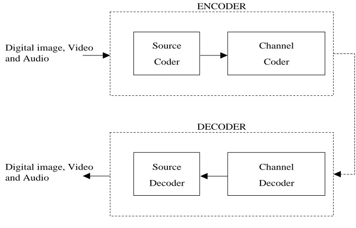
1. A. Explain the steps involved in digital image processing. B.Explain various functional block of digital image processing (OR)

2. Describe the elements of visual perception.

3. Describeimage formation in the eye with brightness adaptation and Discrimination

(OR)

4. Write short notes on sampling and quantization.

5. Describe the functions of elements of digital image processing system with a diagram.

(OR)

6. Explain the basic relationships between pixels? 7. Explain the properties of 2D Fourier Transform.

(OR)

8. ( i )Explain convolution property in 2D fourier transform. (ii) Find F (u) and |F (u)|

9. Explain Fast Fourier Transform (FFT) in detail. (OR)

Page 36 of 137 UNIT II

IMAGE ENHANCEMENT TECHNIQUES

Spatial Domain methods: Basic grey level transformation – Histogram equalization –

Image subtraction – Image averaging –Spatial filtering: Smoothing, sharpening filters –

Laplacian filters – Frequency domain filters: Smoothing – Sharpening filters –

Homomorphic filtering.

1. SPATIAL DOMAIN METHODS

* Suppose we have a digital image which can be represented by a two dimensional random field f(x,y).

* An image processing operator in the spatial domain may be expressed as a mathematical function T







) ,

(x y T f x y

g  as follows.





) ,

(x y T f x y

g 

The operator T applied on f(x,y) may be defined over:

(i) A single pixel (x,y). In this case T is a grey level transformation (or mapping) function.

(ii) Some neighbourhood of (x,y).

(iii) T may operate to a set of input images instead of a single image.

Example 1

The result of the transformation shown in the figure below is to produce an image of higher contrast than the original, by darkening the levels below m and brightening the levels above m in the original image. This technique is known as contrast stretching.

Example 2

m

) (r T s

The result of the transformation shown in the figure below is to produce a binary image.

2. BASIC GRAY LEVEL TRANSFORMATIONS

* We begin the study of image enhancement techniques b y discussing gray-level transformation functions. These are among the simplest of all image enhancement techniques.

* The values of pixels, before and after processing, will be denoted by r and

s, respectively. As indicated in the previous section, these values are related by an expression of the form s=T(r), where T is a transformation that maps a pixel value r

into a pixel value s.

* Since we are dealing with digital quantities, values of the transformation function typically are stored in a one-dimensional a r r a y and the mappings from r to s

are implemented v i a table lookups. For an 8-bit environment, a lookup table containing the values of T will have 256 entries.

* As an introduction to gray-level transformations, consider Fig. 3.3, which shows three basic types of functions used frequently for image enhancement: linear (negative and identity transformations), logarithmic (log and inverse-log transformations), and power-law (nth power and nth root transformations).

* The identity function is the trivial case in which output int e ns it ie s a r e identical to input intensities. It is included in the graph only for completeness.

2.1 Image Negatives

The negative of an image with gray levels in the range [0, L-1] is obtained by using the negative transformation shown in Fig. 3.3, which is given by the expression

m

) (r T s

Page 38 of 137

Reversing the intensity levels of an image in this manner produces the equivalent of a photographic negative. This type of processing is particularly s u i t e d for enhancing w h it e or gray detail embedded i n dark regions of an image, especially when the black areas are dominant i n size. An example is shown in Fig. 3.4. The original image is a digital mammogram s h o w i n g a small lesion. In spite of the fact that the visual content is the same in both images, note how much easier it is to analyze the breast tissue in the negative image in this particular case.

2.2 Log Transformations

The general form of the log transformation shown in Fig. 3.3 is

s = c log (1 + r)

where c is a constant, and it is assumed that r 0.

 The shape of the log curve in Fig. 3.3 shows that this transformation maps a narrow range of low gray-level values in the input image into a wider range of output levels.

 The opposite is true of higher values of input levels. We would use a transformation of this type to expand the values of dark pixels in an image while compressing the higher-level values. The opposite is true of the inverse log transformation.

* Any curve having the general shape of the log functions shown in Fig. 3.3 would accomplish this spreading/compressing of gray levels in an image. In fact, the power-law t rans fo r mat io ns discussed in the next section are much more versatile for this purpose t h