A Novel Iterative Learning Control Design for Linear Discrete Time
Systems Based on A 2D Roesser System
Xinghe Ma, Xuhui Bu
*School of Electrical Engineering & Automation, Henan Polytechnic University, Jiaozuo, China. email: [email protected]
http://dx.doi.org/10.5755/j01.itc.45.4.13391
Abstract. This paper is mainly devoted to the iterative learning control (ILC) design for a class of linear discrete
time systems. By providing a 2D analysis of the learning process, the ILC design for such systems can be transformed into the problem of state feedback or output feedback control for 2-D systems described by Roesser models. Then, a Lyapunov approach can be used to obtain an ILC law that achieves asymptotical convergence of the tracking error. Sufficient stability conditions are provided in terms of linear matrix inequalities, which can determine learning gains as well. The theoretical results are also verified through simulation tests.
Keywords: iterative learning control; 2D Roesser system; linear matrix inequality.
1. Introduction
Many practical control systems have the repetitive operation tasks, such as batch processes [1, 2]. Iterative learning control (ILC) is an effective technique that attempts to achieve a perfect output tracking for such systems over a finite time interval. Motivated by human learning, ILC uses information from previous iterations to improve the input signal of current iteration, and the control objective is achieved finally in the sense that the improvement of learning proceeds from trial to trial. Since the original work in [3], the general area of ILC has been attracted by more and more researchers.
Until now, there are many approaches available with regard to ILC systems. For example, the early contraction mapping approach for linear ILC and nonlinear ILC systems [1, 4, 5], the Lyapunov-based approach for continuous-time systems [6], the super-vector approach for linear discrete-time ILC systems [7, 8], etc. However, there are some essential limits for the above-mentioned approaches. Contraction mapping approach only focuses on the problem of stability or convergence analysis for ILC systems, and does not present the issue of controller design. Lyapunov-based approach is only considered for a class of special continuous-time systems as described in [6]. For linear discrete-time systems, super-vector approach is an effective technique for ILC. This technique reformu-lates the 2D ILC system as 1D system that evolves only in the trial domain. Then, the issue of convergence
*Corresponding author
analysis and controller design can be discussed. For instance, the stability has been analyzed in the frequen-cy domain [9], the time domain [10, 11], and both the frequency and time domains [12]. The design of lifted ILC laws has been studied using 𝐻∞ theory [13, 14], 𝜇
analysis [15] or quadratic cost [16], etc. Even though super-vector approach contributes to the ILC theory, it does not address the computational complexity of the lifted ILC design method that might hamper their real-life application [17, 18]. In the trial domain representation, dimensions of the lifted system matrices (system matrices in the trial domain) are proportional to the number of sampling steps in the trial. Besides computational complexity, another difficulty that might hinder the design of ILC for the case of large trial lengths, is an increased demand for memory locations that are needed to store lifted system matrices.
noted that ILC design with linear matrix inequality (LMI) based on 2-D model have been developed to address the control system stability in both the time and batch directions [23-28]. In [23-25], the ILC design for linear systems can be attributed to the rigorous stability theory of linear repetitive process developed in [23]. Moreover, it is also shown that an LMI re-formulation of the stability conditions for discrete linear repetitive processes leads naturally to design algorithms for con-trol laws to ensure stability along the pass under concon-trol action. In [26], some new concepts and convergence indices are introduced to describe the dynamical beha-viors of the corresponding 2D Roesser system in hori-zontal and vertical propagation directions. Sufficient conditions for stability of the 2D Roesser system are derived, and then a series of new algorithms for ILC design for discrete-time linear systems based on LMI techniques are presented. Under this framework, the ILC design can also be considered for a class of linear systems with time-delay [27], nonlinear systems[28] and advanced PI control [29].
In this paper, a novel ILC design approach based 2-D system theory for a class of discrete time linear systems is presented. After providing a 2D analysis of the learning process, it has been shown that the design problem of an ILC law for such system can be transformed straightforwardly into feedback control problem of 2-D systems described by Roesser models. Here, due to the state signal of ILC system is measu-rable or not, the feedback control for 2-D systems can be designed using state feedback or output feedback. Depending on existed 2-D systems results [30-32], a Lyapunov approach can be employed to develop LMI conditions that guarantee asymptotical convergence for tracking error of the ILC system, and the feasibility and effectiveness of the proposed designs are demonstrated by numerical examples. Compared to the existing methods [23-28], the ILC law is designed based on a simple linear matrix inequality in this paper, resulting in less computation than the existing designs. Besides, when only output signal is available, the proposed design can solve the problem of convex optimization by introducing a new slack variable.
The remainder of this paper is organized as follows. Section 2 presents the description and design objectives of a class of discrete systems together with their transformation into equivalent 2D Roesser systems. In Section 3, a Lyapunov approach for 2D system is employed to develop LMI conditions that guarantee asymptotical convergence of the tracking error for ILC system. Based on the condition, a design approach for ILC law is given. In Section 4, the feasibility and effectiveness of the proposed design algorithms are demonstrated through simulation tests. Finally, the conclusions of this paper are given in Section 5.
2. Problem formulations
We consider the following linear discrete time system
( 1, ) ( , ) ( , ) , ( , ) ( , )
x t k Ax t k Bu t k y t k Cx t k
(1)
where ( , )x t k R u t kn, ( , )Rm, ( , )y t k Rl are state,
input, and output variables, n n, n m
AR R
l n
CR are the matrices describing the system in the
state space. The letterk denotes iteration and t is
discrete time. The system is operated repeatedly in the iteration domain with a desired output y t td( ), [0,N]. Basic assumptions of this system are (i) every operation begins at an identical initial condition, that is
0
(0, )
x k x for all k; (ii) the desired trajectory y td( ) is iteration invariant.
The control objective is to find a control input ( , )
u t k for any 0 n
x R and any initial control
sequence u t( , 0), it generates a output for system such that y t k( , )y td( ) for all t[0, ]N .
A general iterative learning control law can be given as follows:
( , 1) ( , ) ( , ),
u t k u t k u t k (2)
where u t k( , ) denotes modification of the control input.
Remark 1: The ILC updating law (2) means using
the error information from previous trials as efficiently as possible in order to achieve a minimal tracking error in as few iterations as possible. The simplest ILC law is using a proportional-integral derivative learning law, which consists of a proportional, integral and derivative gain on the tracking error to update the system input. More advanced learning laws include plant inversion methods [33], norm-optimal ILC methods [34, 35] or adaptive design methods [36, 37], etc. In this paper, we only consider the simple P-type ILC.
The ILC system (1) and (2) is essentially a 2D system with evolution along two independent axes: time t and iteration k . We can use the 2D analysis
approach to derive an expression for the tracking error and the state error.
Define e t k( , )y td( )y t k( , ) . Using (1) and (2), we can obtain
( , 1) ( , ) ( , ) ( , 1)
( 1, ) ( 1, )
( 1, 1) ( 1, 1)
( , ) ( 1, ),
e t k e t k
y t k y t k
CAx t k CBu t k
CAx t k CBu t k
CA t k CB u t k
(3)
where ( , )t k x t( 1,k 1) x t( 1, )k .
Next, from (1) and (2), the following can also be obtained
( 1, ) ( , 1) ( , )
( , ) ( 1, ).
t k x t k x t k A t k B u t k
(4)
( 1, ) 0 ( , )
( , 1) ( , )
( 1, )
( , )
( 1, ), ( , )
T
t k A t k
e t k CA I e t k
B CB u t k
t k
A B u t k
e t k
(5)
where
0
, .
A B
A B
CA I CB
Now, we consider the following ILC law
1
2
( , 1) ( , 1) ( , )
( , )
( 1, ),
x t k u t k u t k K
x t k K e t k
(6)
where K K1, 2 are designed matrices. (6) can be
rewritten as
1 2
( 1, 1)
( 1, ) [ ] ( 1, )
( , )
( , ) , ( , )
x t k
u t k K K x t k
e t k
t k K
e t k
(7)
where K[K1 K2].
Substituting (7) into (5), we can present the ILC system as a class of 2D systems as follows
( 1, ) ( , )
( , 1) ( , )
( , ) , ( , ) c
t k t k
A BK
e t k e t k
t k A
e t k
(8)
where Ac A BK.
In this case, the problem of ILC design to be addressed in this paper can be transformed as follows: Given a 2-D discrete time system described by (5), design a state feedback controller in the form of (7) such that the resulting closed-loop system (8) is asymptotical stable.
3. Main results
Now, we recall some useful related results on the stability of 2-D discrete systems described by the Roesser model. It has been shown that the stability analysis using Lyapunov functions is efficient to derive sufficient conditions guaranteeing the asymptotic stability for 2-D discrete systems. The well known Lyapunov inequality to test the stability of the 2-D discrete system in (8) is given in the following Lemma.
Lemma 1 [30]. If there exists a positive definite block diagonal matrix
, h T
h v
v
Q
Q Q Q Q
Q
satisfying
- 0, T
c c
A QA Q
then 2-D discrete closed-loop system (8) is asymptotically stable.
The following well-known lemmas are needed in the proof of our main results.
Lemma 2 [38] (Schur Complement). Assume W L, ,
U are given matrices with appropriate
dimensions, where W and U are positive definite symmetric matrices. Then
0
T
L UL W
if and only if
1 0, T
W L
L V
or
1
0. T
V L
L W
Lemma 3 [38]. Given a symmetric matrix n n
R
and two matrices M N, of column
dimension n , there exists a W such that
the following condition holds
+ T+ T T 0,
MWN NW M
if and only if the following projection inequalities with respect to W are satisfied
0, 0,
T T
MM NN
where M and N denote arbitrary bases
of the nullspaces of M and N , respectively.
The following Theorem reveals that the asymptotical stablilty of 2-D discrete closed-loop system (8) can be recast to a matrix inequality feasibility problem.
Theorem 1. Consider the 2-D discrete-time system (8). If there exist a block-diagonal matrix
( , )h v
Pdiag P P with Ph Rn n
and
l l v
PR and matrix S such that
1 1
- ( + ) +
-2 2
- - 0,
1
+ - -
-2
T T T T
c
c c
T T T T
c
S S S A S S P
A S P A S
S S P S A S S
then the closed-loop system (8) is asymptotical stable.
Proof. Matrix inequality (9) can be rewritten as follows:
1 2 1 20 0
-0 - 0 + - - 0
- 0 0
-+ 0 0.
c
T T
c
P I
P A S I I
P I
I
S I A I
I
(10)
Let
1
2 - - , - 0 ,
T T T
c
M I A I N I I
0 0
-0 - 0 ,
- 0 0
P P P
and select the orthogonal complements of M and N( M and N respectively) as:
1 2
0 0
0 , 0 .
- cT 0
I I
M I N I
I A I
Applying Lemma 2 we can obtain
0, 0,
T T
MM NN (11)
that is
1 2
1 2
0 0 - 0
0
0 - 0 0
0
-- 0 0
-0, -T c T c T c c P I I I
M M P I
I A
P I A
P PA
A P P
(12)
and
0 0 - 0
0
0 - 0 0
0 0
- 0 0 0
-2 0 0, 0 -T P I I I
N N P I
I P I P P (13)
Using Lemma 3, we have
-1
- 0. T
c c
PA P A P P (14)
Thus, multiplying the right and the left hand sides of condition (14) by P1 and taking QP1 in the
resulting inequality, we obtain
- 0. T
c c
A QA Q
Using Lemma 1, it is obvious that the asymptotic stability of closed-loop system (8) is guaranteed. This completes the proof of Theorem 1.
To this end, our goal is interested in finding state feedback controller such that the closed loop of 2-D discrete-time system is asymptotically stable. Using Theorem 1 and Ac A BK , the synthesis of feedback controllers can be described to find ( , , )K P S
such that the following matrix inequality holds
1 1
- ( + ) ( + ) +
-2 2
( + ) - -( + ) 0.
1
+ - - ( + )
-2
T T T T
T T T T
S S S A BK S S P
A BK S P A BK S
S S P S A BK S S
(15)
It should be noted that in general the problem of solving numerically (15) for ( , , )K P S is non-convex.
This makes the control problem difficult to solve. However, the introduction of a new variable Y in (15),
such that YKS leads to a convex sufficient condition
in terms of LMI as in the following theorem
Theorem 2. If there exist positive definite
( , )h v
Pdiag P P with Ph Rn n
, l l
v
P R
and matrices S , Y such that
1 1
- ( + ) ( + ) +
-2 2
+ - -( + ) 0,
1
+ - -( + )
-2
T T T
T T T
S S AS BY S S P
AS BY P AS BY
S S P AS BY S S
(16)
then 2-D discrete closed-loop system (8) is asymptotical stable. In this situation, a suitable control law for (7) can be given as -1
KYS .
Remark 2: Theorem 2 provides an LMI condition for
the ILC convergence, which is expressed in terms of learning gains and plant model parameters. This falls into the category of ILC where a convergence condition is given with respect to known plant knowledge. But in contrast, this LMI condition provides a direct approach to determine learning gains.
Next, we extend the above analysis to the case of unavailable state .
In ILC updating law (6), both output signal and state signal of the ILC system are used. However, state signals may be measurable or difficult to be measured in many practical systems. In this case, only output signal can be used. The ILC law can be constructed as Arimoto P-type updating law given by
( , 1) ( , ) ( 1, ),
u t k u t k e t k (17)
where is the learning gain matrix.
We add an output equation for 2D system (5) as follows
( , )
( , ) ,
( , )
t k y t k C
e t k
where
1 n n
l l
C
0
. It can be easy obtained that
( , )
( , )
y t k
e t k
0
. Then the problem of ILC design can
be transformed as: Given a 2-D discrete time system described by
( 1, ) ( , )
( 1, )
( , 1) ( , )
( , )
( , ) ,
( , )
t k t k
A B u t k
e t k e t k
t k
y t k C
e t k
(18)
design an output feedback controller in the form of ( 1, ) ( , ),
u t k Ky t k
(19)
such that the resulting closed-loop system is asymptotically stable.
Denote K2[0n L] . From (17), (18) and (19), we have
2 .
K KC
Substituting (19) into (18), we can present the ILC system as a 2-D discrete closed-loop system given by
( 1, ) ( , )
( , 1) ( , )
( , ) , ( , ) c
t k t k
A BKC
e t k e t k
t k A
e t k
(20)
where Ac A BKC.
Using Theorem 1, the synthesis of output feedback controller can be described to find ( , , )K P S such that
the following matrix inequality holds
1 1
- ( + ) ( + ) +
-2 2
( + ) - -( + ) 0.
1
+ - - ( + )
-2
T T T T
T T T T
S S S A BKC S S P
A BKC S P A BKC S
S S P S A BKC S S
(21)
We note that the problem of solving numerically (21) is non-convex. This makes the matrix inequality difficult to be solved.
We introduce a new slack variable G in (21), such that KCSKGC. Then, a convex sufficient condition
of solving (21) can be given in terms of LMI.
Theorem 3. If there exist positive definite
( , )h v
Pdiag P P with Ph Rn n
, l l
v
PR
and matrices S , G , Y such that
1 1
- ( + ) +
-2 2
- -( ) 0,
1
+ - -
-2
+ 0,
,
T T T T T T T
T T T T T T T
T
S S S A C Y B S S P
AS BYC P AS BYC
S S P S A C Y B S S
G G
CS GC
(22)
then 2-D discrete closed-loop system (20) is asymptotical stable, and a feasible control law for (19) can be given as -1
KYG . In this situation, the ILC
gain matrix in (17) can be selected as -1
2 .
K YG C
Remark 3. It is worthy pointing out that the equality constraint CSGC is satisfied by the slack variable G. The invertibility of matrix G is guaranteed by the
condition +G GT 0.
Remark 4. The proposed approach is systematic for ILC controller design. This result can be extended to more complex systems (systems with time-delays, uncertainties, etc) and more special performance design such as H,H2.
4. Numerical Examples
In this section, an example is provided to illustrate the validity of our design. Let us consider the following discrete-time system
0.25 0.6 1
( , 1) ( , ) ( , ),
0.6 0 0
( , ) 1 1.3 ( , ).
x k t x k t u k t
y k t x k t
(23)
The desired repetitive reference trajectory is: ( ) sin(8.0 / 50), 0,1, 2, ,100. d
y t t t
For the initial state, it is assumed that
1(0, ) 2(0, ) 0
x k x k for all k. The ILC law is applied
by adopting the zero initial control input ( ,0) 0u t for
all t. Using system parameters in (23), the matrices in
(5) can be calculated with the following parameters
0.25 0.6 0 1
0.6 0 0 , 0
0.53 0.6 1 1
A B
.
Then, the state is measurable and immeasurable are separately considered .
Case 1 state is measurable
In this case, the ILC updating law is given as
1 2
( , 1) ( , ) ( , 1) ( , ) ( 1, )
u t k u t k K x t k x t k K e t k ,
and the state feedback controller matrix for 2D system is K[K1 K2] . Using Theorem 2, we know that once the LMI (16) is feasible, the learning gain matrix can be determined by -1
KYS , and the closed-loop
system is asymptotically stable. With the help of the Matlab LMI toolbox, a feasible solution for the LMI (16) can be obtained as follows
-5.2144 -21.5447 4.9220 ,
21.0390 5.2645 -15.32245.2645 36.8271 -3.4198 , -15.3224 -3.4198 11.5909
Y
S
28.3967 7.9373 -20.7490
7.9373 57.4566 -5.2486 .
-20.7490 -5.2486 15.6582
P
Hence, the ILC gain matrix can be selected as
-1
2.2247 -0.6072 3.1864 .
KYS
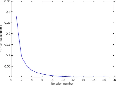
The results of simulation are shown in Fig. 1. Fig. 1 (a)-(d) give system output at the 2nd, 3rd, 5th, 10th iterations (solid line) and the desired output trajectory (dash line). Fig. 2 gives the max tracking error on the iteration domain. It can be observed that by using the proposed iterative learning control law, we can guarantee the asymptotic convergence of the tracking error for all t[1,100].
Case 2 State is immeasurable
In this case, it is assumed that the state signal is immeasurable, and the ILC updating law is given as
( , 1) ( , ) ( 1, )
u t k u t k e t k . We add an output
equation for 2D system as (18), and the matrix C is
selected as
0
0
1
C
.
Using Theorem 3, we know that once the LMI (22) is feasible, the gain matrix for 2D system can be determined by -1
KYG , and then the closed-loop
(a)
(b)
(c)
(d)
Figure 1. Simulation results for Case 1: (a) output profiles at 2nd iteration; (b) output profiles at 3rd iteration; (c) output profiles at 5th iteration; (d) output profiles at 10th iteration
Figure 2. The max tracking error for Case1
0 10 20 30 40 50 60 70 80 90 100
-1.5 -1 -0.5 0 0.5 1 1.5
step
O
u
tp
u
t
desired trajectory yk(t) at 2th iteration
0 10 20 30 40 50 60 70 80 90 100
-1.5 -1 -0.5 0 0.5 1 1.5
step
O
u
tp
u
t
desired trajectory yk(t) at 3th iteration
0 10 20 30 40 50 60 70 80 90 100
-1.5 -1 -0.5 0 0.5 1 1.5
step
O
u
tp
u
t
desired trajectory yk(t) at 5th iteration
0 10 20 30 40 50 60 70 80 90 100
-1.5 -1 -0.5 0 0.5 1 1.5
step
O
u
tp
u
t
desired trajectory yk(t) at 10th iteration
0 2 4 6 8 10 12 14 16 18 20
0 0.05 0.1 0.15 0.2 0.25 0.3 0.35
iteration number
Th
e
m
a
x
t
ra
c
k
in
g
e
rr
o
system (20) is asymptotically stable. With the help of the Matlab LMI toolbox, a feasible solution can be obtained as
1.0 004* 0 -6.7863 0.0091 ,
2.0199 -0.0070 -1.4150 1.0 003 * -0.0070 8.1148 0.0568 ,
-1.4150 0.0568 1.0347
Y e
S e
0.3183 0.0253 -0.2279
1.0 004 * 0.0253 1.3932 -0.0113 ,
-0.2279 -0.0113 0.1687
P e
5.4964 -0.0007 -0.1415
1.0 004 * -0.0007 0.8115 0.0057 .
-0.1415 0.0057 0.1035
G e
Then, the 2D output feedback gain matrix is:
-1
0.0135 -8.3668 0.5657 ,
KYG
and
-1
2 0 0 0.5657 ,
K YG C
hence, ILC gain matrix for (17) is =0.5657 . The simulation results are shown in Fig. 3. Fig. 3 (a)-(d) also give system output at the 2nd, 3rd, 5th, 10th iterations (solid line) and the desired output
trajectory (dash line), and Fig. 4 gives the max tracking error on the iteration domain. Clearly, the ILC system is stable also in this case. Note that in existing contraction mapping approach, a sufficient stability condition of P-type ILC (17) for linear discrete system (1) is ICB 1 . When =0.5657 , the condition
0.4343 1
ICB is obvious satisfied.
Compa-ring the simulation results of two cases, we can also observe that when the state signal is available, the fast convergence speed and small transient error can be obtained.
5. Conclusions
In this paper, an ILC design approach for a class of linear discrete time systems has been presented. After providing a 2D analysis of the learning process, it has been shown that the design problem of ILC law for such system can be transformed straightforwardly into state feedback or output feedback control problem of 2-D systems described by Roesser models. Then, a Lyapunov approach has been employed to develop LMI conditions that guarantee asymptotical convergence of the tracking error. It is also shown that the solution can be recast as a convex optimization under LMI form. The theoretical results have been verified through simulation tests.
(a)
(b)
(c)
(d)
Figure.3. Simulation results for Case 2: (a) output profiles at 2nd iteration; (b) output profiles at 3rd iteration; (c) output profiles at 5th iteration; (d) output
profiles at 10th iteration
0 10 20 30 40 50 60 70 80 90 100 -1.5
-1 -0.5 0 0.5 1 1.5
step
O
u
tp
u
t
desired trajectory yk(t) at 2th iteration
0 10 20 30 40 50 60 70 80 90 100
-1.5 -1 -0.5 0 0.5 1 1.5
step
O
u
tp
u
t
desired trajectory yk(t) at 3th iteration
0 10 20 30 40 50 60 70 80 90 100 -1.5
-1 -0.5 0 0.5 1 1.5
step
O
u
tp
u
t
desired trajectory y
k(t) at 5th iteration
0 10 20 30 40 50 60 70 80 90 100 -1.5
-1 -0.5 0 0.5 1 1.5
step
O
u
tp
u
t
Figure.4. The max tracking error for Case 2
Acknowledgement
This work was supported by the National Natural Science Foundation of China (Nos. 61573129, 61203065, U1404522), the Program for Science & Technology Innovation Talents in Universities of Henan Province (16HASTIT046), the Fundamental Research Funds for the Universities of Henan Province, the program of Key Young Teacher of Higher Education of Henan Province (2014GGJS-041), the program of Key Young Teacher of Henan Polytechnic University and the Doctoral Fund Program of Henan Polytechnic University (B2012-003).
References
[1] C. L. Li, L. Y. Li. An efficient scheduling strategy for
batch processing applications in mobile cloud: model and algorithm. Information Technology and Control,
2015, Vol. 44, No. 1, 7-19.
[2] V. Galvanauskas. Adaptive PH control system for
fed-batch biochemical processes. Information Technology and Control, 2009, Vol. 38, No. 3, 225-231.
[3] S. Arimoto, S. Kawamura, F. Miyazaki. Bettering
operation of robots by learning. J. of Robotic Systems, 1984, Vol. 1,123-140.
[4] Z. Bien, J. X. Xu. Iterative learning control: Analysis,
design, integration and applications. Dordrecht: Kluwer Academic Publishers. 1998
[5] Y. Chen, C. Wen. Iterative learning control: Conver-gence, robustness and applications. Lecture notes in control and information sciences. Berlin: Springer. 1999.
[6] A.Tayebi. Analysis of two particular iterative learning
control schemes in frequency and time domains.
Automatica, 2007, Vol. 43, No. 9, 1565-1572
[7] S. Gunarsson, M. Norrlof. On the design of ILC
algo-rithms using optimization. Automatica, 2001, Vol. 37, No. 12, 2011-2016.
[8] K. L. Moore. An observation about monotonic
conver-gence in discrete-time, P-type iterative learning control. In: Proc. 2001 IEEE Int. Symp. Intell. Control, Mexico, Sep., 2001, pp. 45-49.
[9] D. A. Bristow, A. G. Alleyne. Monotonic convergence
of iterative learning control for uncertain systems using a time-varying filter. IEEE Trans. Autom. Control, 2008, Vol. 53, No. 2, 582-585.
[10] H. S. Ahn, K. L. Moore, Y. Chen. Stability analysis of
discrete-time iterative learning control systems with interval uncertainty. Automatica, 2007, Vol. 43, No. 5, 892-902.
[11] H. S. Ahn, K. L. Moore, Y. Chen. Monotonic
conver-gent iterative learning controller design based on inter-val model conversion. IEEE Trans. Autom. Control, 2006, Vol. 51, No. 2, 366-371
[12] M. Norrlof, S. Gunnarsson. Time and frequency
do-main convergence properties in iterative learning con-trol. Int. J. Control, 2002, Vol. 75, No. 14, 1114–1126. [13] K. L. Moore, H.-S. Ahn, Y. Chen. Iteration domain
𝐻∞-optimal iterative learning controller design. Inter-national Journal of Robust and Nonlinear Control,
2008, Vol. 18, No. 10, 1001-1017.
[14] X. H. Bu, Z. S. Hou, F. S. Yu, F. Z. Wang. H∞ ite-rative learning controller design for a class of discrete-time systems with data dropouts. International Journal of Systems Science, 2014, Vol. 45, No. 9, 1902-1912.
[15] J. Van De Wijdeven, T. Donkers, O. Bosgra. Iterative
learning control for uncertain systems: robust monoto-nic convergence analysis. Automatica, 2009, Vol. 45, No. 10, 2383-2391.
[16] D. A. Bristow. Weighting matrix design for robust
mo-notonic convergence in norm optimal iterative learning control. In: Proceedings of the American Control Conference, 2008, pp. 4554- 4560.
[17] A. Haber, R. Fraanje, M. Verhaegen. Linear
compu-tational complexity robust ILC for lifted systems. Auto-matica, 2012, Vol. 48, No. 6, 1102-1110
[18] X. H. Bu, H. W. Zhang, Y. Z. Song, F. S. Yu. Hinf ILC Design for Discrete Linear Systems with Packet Dropouts and Iteration-Varying Disturbances. Discrete Dynamics in Nature and Society, 2014, Vol. 2014, 1-11.
[19] J. E. Kurek, M. B. Zaremba. Iterative learning control
synthesis based on 2-D system theory. IEEE Trans. Autom. Control, 1993, Vol. 38, No. 1, 121-125.
[20] X. D. Li, T. W. S. Chow, J. K. L. Ho. 2-D system
theory based iterative learning control for linear conti-nuous systems with time delays. IEEE Trans. Circuits Syst. I, Regul. Pap., 2005, Vol. 52, No. 7, 1421-1430.
[21] T. W. S. Chow, Y. Fang. An iterative learning control
method for continuous-time systems based on 2-D system theory. IEEE Trans. Circuits Syst. I, Fundam. Theory Appl., 1998, Vol. 45, No. 6, 683-689.
[22] S. S. Saab. A discrete-time stochastic learning control
algorithm. IEEE Trans. Autom. Control, 2001, Vol. 46, No. 6, 877-887.
[23] E. Rogers, K. Galkowski, D. H. Owens.Control
Sys-tems Theory and Applications for Linear Repetitive Pro-cesses. Berlin, Germany: Springer-Verlag, 2001.
[24] M. French, E. Rogers, H. Wibowo, D. H. Owens. A
2D systems approach to iterative learning control based on nonlinear adaptive control techniques. In: Proc. 2001 IEEE Int. Symp. on Circuits Syst., Sydney, Australia, May 6-9, 2001, pp. 429-432.
[25] E. Rogers, K. Galkowski, A. Gramacki, J. Gramacki,
D. H. Owens. Stability and controllability of a class of 2-D linear systems with dynamic boundary conditions.
IEEE Trans. Circuits Syst. I: Fundam. Theory Appl., 2002, Vol. 49, No. 2, 181-195.
[26] J. Shi, F. Gao, T.-J. Wu. Robust design of integrated
feedback and iterative learning control of a batch pro-cess based on a 2D Roesser system. J. Process Control, 2005, Vol. 15, No. 8, 907-924.
0 2 4 6 8 10 12 14 16 18 20
0 0.1 0.2 0.3 0.4 0.5 0.6 0.7
iteration number
Th
e
m
a
x
t
ra
c
k
in
g
e
rr
o
[27] T. Liu, F. Gao. Robust two-dimensional iterative lear-ning control for batch processes with state delay and time-varying uncertainties. Chemical Engineering Science, 2010, Vol. 65, No. 23, 6134-6144.
[28] T. Liu, Y. Wang. A synthetic approach for robust
constrained iteration learning control of piece affine batch processes. Automatica, 2012, Vol. 48, No. 11, 2762-2775.
[29] Y. Wang, Y. Yang, Z. Zhao. Robust stability analysis
for an enhanced ILC-based PI controller. Journal of Process Control, 2013, Vol. 23, No. 2, 201-214.
[30] C. Du, L. Xie, C. Zhang.H∞ control and robust
stabili-zation of two-dimensional systems in Roesser models.
Automatica, 2001, Vol. 37, No. 2, 205-211.
[31] M. Nachidi, F. Tadeo, A. Hmamed, M. Alfidi, Static
Output-feedback controller design for Two-Dimen-sional Roesser models. International Journal of Science and Techniques of Automatic Control, 2008, Vol. 2, No. 2, 738-747.
[32] A. Dhawan, H. Kar. An LMI approach to robust
opti-mal guaranteed cost control of 2-D discrete systems described by the Roesser model. Signal Processing,
2010, Vol. 90, No. 9, 2648-2654.
[33] K. Kinosita, T. Sogo, N. Adachi. Iterative learning control using adjoint systems and stable inversion.
Asian J. Control, 2002, Vol. 4, 60-67.
[34] V. Hatzikos, J. Hatonen, D. H. Owens. Genetic
algo-rithms in norm-optimal linear and non-linear iterative learning control. Int. J. Control, 2004, Vol. 77, No. 2, 188-197.
[35] N. Amann, D. H. Owens, E. Rogers. Predictive
opti-mal iterative learning control. Int. J. Control, 1998, Vol. 69, No. 2, 203-226.
[36] R. H. Chi, Z. S. Hou, J. X. Xu. Adaptive ILC for a class of discrete-time systems with iteration-varying trajectory and random initial condition. Automatica, 2008, Vol. 44, No. 8, 2207-2213
[37] W. S. Chen, J. M. Li, J. Li. Practical adaptive iterative learning control framework based on robust adaptive approach. Asian Journal of Control, 2011, Vol. 13, No. 1, 85-93.
[38] S. Boyd, L. E. Ghaoui, E. Feron, V. Balakrishnan.
Linear matrix inequalities in system and control theory. SIAM, Philadelphia, PA: SIAM, 1994.