Asynchronous Proximal Stochastic Gradient Algorithm for Composition Optimization Problems

(1)

The Thirty-Third AAAI Conference on Artificial Intelligence (AAAI-19)

Asynchronous Proximal Stochastic Gradient

Algorithm for Composition Optimization Problems

Pengfei Wang,

1,2

_{Risheng Liu,}

3

_{Nenggan Zheng,}

1∗

_{Zhefeng Gong}

4 1_{Qiushi Academy for Advanced Studies, Zhejiang University, Hangzhou, Zhejiang, China} 2_{College of Computer Science and Technology, Zhejiang University, Hangzhou, Zhejiang, China} 3_{International School of Information Science & Engineering, Dalian University of Technology, Liaoning, China}

4_{Department of Neurobiology, Zhejiang University School of Medicine, Hangzhou, Zhejiang, China}

{pfei, zng, zfgong}@zju.edu.cn, [email protected]

Abstract

In machine learning research, many emerging applications can be (re)formulated as the composition optimization prob-lem with nonsmooth regularization penalty. To solve this problem, traditional stochastic gradient descent (SGD) algo-rithm and its variants either have low convergence rate or are computationally expensive. Recently, several stochastic composition gradient algorithms have been proposed, how-ever, these methods are still inefficient and not scalable to large-scale composition optimization problem instances. To address these challenges, we propose an asynchronous par-allel algorithm, named Async-ProxSCVR, which effectively combines asynchronous parallel implementation and variance reduction method. We prove that the algorithm admits the fastest convergence rate for both strongly convex and gen-eral nonconvex cases. Furthermore, we analyze the query complexity of the proposed algorithm and prove that linear speedup is accessible when we increase the number of pro-cessors. Finally, we evaluate our algorithm Async-ProxSCVR on two representative composition optimization problems in-cluding value function evaluation in reinforcement learn-ing and sparse mean-variance optimization problem. Exper-imental results show that the algorithm achieves significant speedups and is much faster than existing compared methods.

Introduction

Composition optimization problem proposed recently by Wang et al. (Wang, Fang, and Liu 2014) arises in many important applications including reinforcement learning (Wang, Liu, and Tang 2017), statistical learning (Hinton and Roweis 2003), risk management (Shapiro, Dentcheva, and Ruszczy´nski 2009), and multi-stage stochastic programming (Shapiro, Dentcheva, and Ruszczy´nski 2009). In this paper, we study the finite-sum scenario for the regularized com-position optimization problem whose objective function is the composition of two finite-sum functions plus a possibly nonsmooth regularization term, i.e.,

min

xPRNHpxq “fpxq `hpxq, (1)

∗

Corresponding author

where

fpxq “ 1

n1

ÿ

i“1

Fip

1

n2

ÿ

j“1

Gjpxqq, (2)

where Gj : RN Ñ RM, Fi : RM Ñ R, and

f : _RN

Ñ R are continuously differentiable functions.

We denote Gpxq :“ _n1

2

řn2

j“1Gjpxq, y :“ Gpxq, and

Fpyq:“ _n1

1

řn1

i“1Fipyq. And we callGpxqthe inner

func-tion and Fpyq the outer function. Often fpxq is used as the empirical risk approximation to the composition of two expected-value functionEiFipEjGjpxqq. The regularization

h:RN ÑRYt`8uis an extended real-valued closed con-vex but possibly nonsmooth function, which is often used to constrain the capacity of the hypothesis space.

In general, problem (1) is substantially more chal-lenging than its non-composition counterpart, i.e., empiri-cal risk minimization (ERM) problem (Friedman, Hastie, and Tibshirani 2001) with the finite-sum form fpxq “

1{nřn_i_“1Fipxq. On the one hand, the composition objec-tive is nonlinear with respect to the joint distribution of data indices pi, jq, which leads to the difficulty of an unbiased sampling for estimating the full gradient ∇fpxq. On the other hand, the two finite-sums structure causes unprece-dented computational challenges for traditional stochastic gradient methods in solving problem (1). For example, to apply stochastic gradient descent (SGD) method, we need to computepBGjpxqqT∇FipGpxqqin each iteration. The in-ner function Gpxqis computationally expensive with per-iteration queries proportional ton2.

(2)

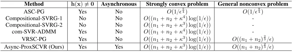
Table 1: Comparisons of query complexity for existing stochastic composition gradient algorithms including ASC-PG (Wang, Liu, and Tang 2017), Compositional-SVRG-1 (Lian, Wang, and Liu 2017), Compositional-SVRG-2 (Lian, Wang, and Liu 2017), com-SVR-ADMM (Yu and Huang 2017), VRSC-PG (Huo, Gu, and Huang 2018), and our proposed Async-ProxSCVR algorithm.n1denotes the number of outer component functions.n2denotes the number of inner component functions.κis the

condition number defined in section Convergence Analysis.

Method hpxq ı0 Asynchronous Strongly convex problem General nonconvex problem

ASC-PG Yes No Op1{54_q O_p1_{

9

4_q

Compositional-SVRG-1 No No Oppn1`n2`κ4qlogp1{qq

-Compositional-SVRG-2 No No Oppn1`n2`κ3qlogp1{qq

-com-SVR-ADMM Yes No Oppn1`n2`κ4qlogp1{qq

-VRSC-PG Yes No Oppn1`n2`κ3qlogp1{qq Oppn1`n2q 2

3_{_q

Async-ProxSCVR (Ours) Yes Yes Oppn1`n2`κ3qlogp1{qq Oppn1`n2q 2

3_{_q

VRSC-PG (Huo, Gu, and Huang 2018). Compositional-SVRG-1 and Compositional-SVRG-2 are designed for prob-lem (1) wherehpxq ” 0, while VRSC-PG can deal with problem (1) with nonsmooth regularization term. In addi-tion, (Yu and Huang 2017) proposes an algorithm, com-SVR-ADMM, which combines ideas of SVRG and ADMM for the composition optimization problem (1) with linear constraints. The query complexity1of these stochastic com-position gradient algorithms are shown in Table 1. Although these existing methods for problem (1) may have good the-oretical guarantees and analytical properties, they are inher-ently non-parallel (i.e., sequential) which are not scalable to modern large-scale composition optimization problems.

Another approach to improve the efficiency for solving problem (1) is the asynchronous parallel implementation, which has been successfully applied to speedup many state-of-the-art algorithms (Recht et al. 2011; Reddi et al. 2015; Zhang and Kwok 2014; Liu and Wright 2014; Liu et al. 2015). However, existing asynchronous parallel algorithms focus on solving the ERM problem. When directly utilizing existing asynchronous parallel methods, e.g., HOGWILD! (Recht et al. 2011) and Async-ProxSVRG (Meng et al. 2017) to solve problem (1), the inner functionGpxqand its Jacobi matrixBGpxqstill need to be computed in each itera-tion, which usually costs too much time and is inefficient for practical applications.

To fill this important gap, in this paper, we propose an asynchronous proximal variance reduction based algorithm, Async-ProxSCVR, for the composition optimization prob-lem (1) with nonsmooth regularization term. We provide the convergence guarantees of the algorithm for both strongly convex and general nonconvex cases. We also prove that the total query complexity of our asynchronous algorithm would be comparable to its serial counterpart, which indicates a lin-ear speedup. Our main contributions are listed as follows: • By effectively combining the asynchronous parallel

im-plementation with the variance reduction method, we develop an asynchronous proximal variance reduction method, Async-ProxSCVR, for problem (1) with nons-mooth regularization. Our method is time-efficient with low computational cost per iteration.

1

The query complexity is measured in terms of the total number of component function queries to find an-accurate solution.

• We prove that Async-ProxSCVR achieves a query com-plexity ofOppn1`n2`κ3qlogp1{qqfor strongly

con-vex case and Oppn1 `n2q 2

3_{_q for general nonconvex

case, which match the best results for existing stochastic composition algorithms. Furthermore, our analysis show that Async-ProxSCVR can achieve linear speedup with respect to the number of processors.

• We test our asynchronous parallel algorithm on two rep-resentative composition optimization problems including value function evaluation in reinforcement learning and sparse mean-variance optimization. The experimental re-sults prove that our method achieves significant speedup and can converge faster than other existing stochastic composition gradient methods.

Notations

Throughout this paper, we use the following notations: • x˚_P

RN denotes the optimal solution for problem (1).

• || ¨ ||denotes the Euclidean norm|| ¨ ||2.

• BGjpxqdenotes the Jacobi matrix of multivariate function Gjp¨qat pointx.

• ∇Fipyq denotes the derivative function of multivariate

functionFip¨qat pointy.

Related Work

(3)

the Async-ProxSVRG requires highOpn2qqueries per

iter-ation which are computiter-ationally expensive.

Variance Reduction Methods. To alleviate the adverse effect of randomness inherent in stochastic gradient al-gorithms, several variance reduction methods have been proposed, e.g., SVRG (Johnson and Zhang 2013), SAG (Schmidt, Le Roux, and Bach 2017), SDCA (Shalev-Shwartz and Zhang 2013) and SAGA (Defazio, Bach, and Lacoste-Julien 2014). Due to its low memory overhead, we focus on the SVRG method, which is initially used to solve the ERM problem with the finite-sum form fpxq “

1{nřn_i_“1Fipxq. The SVRG algorithm has double loops.

More specifically, at thesth_{epoch, the SVRG keeps a}

snap-shot of iteration vector rx

s _{and compute its full gradient}

∇fpx_rsq. In thekth_{inner loop, the SVRG compute gradient}

estimator based on the following update rule:

vs_k“∇Fikpx

s

kq ´∇Fikprx

s

q `∇fpxr s

q, (3)

whereikis randomly selected fromrns. This update rule has a lower iteration cost, because there is no need to calculate the full gradient in each iteration. The gradient estimator is unbiased, i.e.,Ervs

ks “∇fpxskq. Besides, the variance of the

gradient estimator induced by the random sampling is upper bounded (Johnson and Zhang 2013):

Er||v_ks||2s ď4Lfrfpxs_kq ´fpx˚

q `fpxr s

q ´fpx˚

qs. (4)

Whenxs

kandxrapproach the optimal solutionx

˚_{, the}

vari-ance of gradient goes to0. Furthermore, The SVRG method has a provably faster convergence rate, i.e.,Opnlog1qfor

strongly convex case (Johnson and Zhang 2013) andOpn

2 3

q

for nonconvex case (Reddi et al. 2016). Recently, many vari-ants of the SVRG method have achieved great success, e.g., the proximal SVRG method (Xiao and Zhang 2014), the asynchronous SVRG method (Reddi et al. 2015) and the dis-tributed SVRG method (Lee et al. 2015). In our method, we introduce a SVRG-based compositional variance reduction method to effectively solve the composition problem (1).

Asynchronous Proximal Stochastic

Compositional Variance Reduction Algorithm

In this section, we propose Async-ProxSCVR to solve the composition optimization problem (1) with nonsmooth reg-ularization penalty. Our proposed Async-ProxSCVR ex-ploits the asynchronous parallel scheme and compositional variance reduction method, which is significantly different from existing works (Fang and Lin 2017; Huo, Gu, and Huang 2018; Yu and Huang 2017) as discussed before.

1. For asynchronous parallel implementation, we use the shared memory multi-core computational model that mul-tiple processors have free access to the vectorxstored in the shared memory and independently execute the itera-tive task concurrently without using any locks2_.

2

This may result in theinconsistent reading and writing, which makes the convergence analysis of the proposed Async-ProxSCVR method more challenging.

Algorithm 1:Async-ProxSCVR

Input:initial vectorx_r0_{, step size}_η_{, number of inner}

loopsm, number of outer loopsS, size of mini-batchA,BandI.

Output:x_rS_and_x

a, wherexais uniformly selected

fromttxs_kum_k_“0´1uS_s_“0´1.

fors“0,1,¨ ¨ ¨, S´1do

xs

0“xr

s_;

// n2 queries

Gprx

s

q “_n1

2

řn2

j“1Gjprx

s_q;

// n2 queries

BGprx s

q “_n1

2

řn2

j“1BGjpxr

s_q;

// n1 queries

∇fpx_rsq “ pBGpx_rsqqT_n1

1

řn1

i“1∇FipGprx

s_qq;

Parallel Computation on Multiple Threads fork“0,1,¨ ¨ ¨, m´1do

Readxs_D_p_k_qfrom the shared memory; Randomly chooseAkĂ rn2swith|Ak| “A;

// 2A queries

ComputeGˆs

Dpkqfrom Eq.(6);

Randomly chooseBkĂ rn2swith|Bk| “B;

// 2B queries

ComputeBGˆs

Dpkqfrom Eq.(7);

Randomly chooseIk Ă rn1swith|Ik| “I;

// 2I queries

Computevs

kfrom Eq.(8);

Updatexs_k_`1“Proxηhpxsk´ηv s

kq;

end

Option I:x_rs`1“xs_m;

Option II:x_rs`1

“_m1 řm_k_“1xs

k;

end

2. For compositional variance reduction method, consid-ering the two finite-sums structure in problem (1), our proposed Async-ProxSCVR employs variance reduction method to estimate the inner function Gp¨q, the partial gradient of inner functionBGp¨q, and the gradient of full function∇fp¨qwith low per-iteration queries.

More specifically, following the SVRG method (Johnson and Zhang 2013), the proposed Async-ProxSCVR algorithm has two-layer loops. At the beginning of outer epochs, we compute the full gradient∇fprx

s

qat the snapshot pointxr

s_:

∇fprx s

q “ pBGprx s

qqT∇FpGpxr s

qq, (5)

whereGpx_rs

q “ _n1

2

řn2

j“1Gjpxr

s

qdenotes the value of the inner function andBGprx

s

q “_n1

2

řn2

j“1BGjprx

s

qdenotes the full gradient of inner function. Computing the full gradient ∇fpxr

s

qrequires a total ofpn1`2n2qqueries.

In the inner loop, each processor repeatedly runs the fol-lowing steps:readthe iteration vector from the shared

mem-ory,compute the gradient estimator, and then update the

(4)

Bk Ă rn2s being random sampling sets, |Ak| “ A and

|Bk| “ B, we compute the estimated values ofGp¨qand BGp¨q at the iteration vector xs

Dpkq read from the shared

memory:

ˆ

Gs_D_p_k_q:“ 1

A ÿ

1ďjPA

pGA_k_r_j_spxs_D_p_k_qq ´GA_k_r_j_spx_rsqq

`Gp_rxsq, (6)

BGˆs_D_p_k_q:“ 1

B ÿ

1ďjďB

pBGBkrjspx

s

Dpkqq ´ BGBkrjspxr s

qq

` BGpx_rsq, (7)

whereAkandBkare independent. Note that the query

com-plexities of computingGˆs

DpkqandBGˆ

s

Dpkqare independent

of the number of inner component functions, i.e.,n2.

Now, we compute the gradient estimator as follows:

vks:“

1

I ÿ

ikPIk

ppBGˆs_D_p_k_qqT∇Fi_kpGˆs_D_p_k_qq

´ pBGpxr s

qqT∇Fi_kpGpxr s

qqq `∇fprx s

q, (8)

whereIk Ă rn1sis random sampling set with|Ik| “I.

Fi-nally, we update the iteration vectorxs

t`1through a proximal

operator:

xs_k_`1“Proxηhpxsk´ηv

s

kq, (9)

whereηis the learning rate. For each inner loop, computing the gradient estimator requires2pA`B`Iqqeuries. After

minner iterations, we update the snapshot pointx_rs`1_based

on Option I or Option II for the next epoch. The detailed Async-ProxSCVR algorithm is presented in Algorithm 1.

In the inner loop, we maintain the iteration counterkto track the number ofupdateoperations. Since update hap-pens asynchronously, there will generally be a delay be-tween the current iteration vector and the iteration vector used to calculate the gradient estimator. In Eq.(6), Eq.(7), and Eq.(8), we useDpkqto denote the iteration counter cor-responding to the time that the iteration vector in the shared memory is read at thekth_{iteration. The iteration value}_xs

Dpkq

can be represented as below:

xs_D_p_k_q“xsk´τk`

ÿ

hPJpkq

pxh`1´xhq, (10)

whereJpkq Ă tk´τk,¨ ¨ ¨, k´1u, andτkdenotes the time delay of the gradient estimator at thekth_iteration.

Note that the gradient estimatorv_ks in Algorithm 1 is a biased estimation of∇fpxs

Dpkqqsignificantly different from

the unbiased estimation in standard SVRG method. Hence, the convergence analysis of Async-ProxSCVR is more com-plex than existing asynchronous variance reduction algo-rithms (Reddi et al. 2015; Meng et al. 2017).

Convergence Analysis

We now proceed to analyze the convergence behavior and evaluate the query complexity of our proposed Async-ProxSCVR for both strongly convex and general

noncon-vex cases. We first make some commonly used assump-tions in the literatures of composition optimization prob-lems (Lian, Wang, and Liu 2017; Huo, Gu, and Huang 2018; Yu and Huang 2017).

Assumption 1(Lipschitzian Gradients). Fori P rn1s,j P

rn2s, there exist constants0ăLF, LG, Lf ă 8such that

||∇Fipy1q ´∇Fipy2q|| ďLF||y1´y2||,@y1, y2PRM,

||BGjpx1q ´ BGjpx2q|| ďLG||x1´x2||,@x1, x2PRN,

||pBGjpx1qqT∇FipGpx1qq ´ pBGjpx2qqT∇FipGpx2qq||

ďLf||x1´x2||,@x1, x2PRN.

Assumption 2(Bounded Gradients). ForiP rn1s,jP rn2s,

there exist some constants0ăBF, BGă 8such that

||∇Fipyq|| ďBF,||BGjpxq|| ďBG,@xPRN,@yPRM.

Assumption 3(Bounded Delay). There exists a delay

pa-rameterτsuch that the random delay variablesτkare upper

bounded byτ, i.e.,τk ďτin Async-ProxSCVR.

Letσ :“B4

GL2F{A`BF2L2G{B. According to

Assump-tion 1, we can immediately arrive at a corollary thatfpxqis

Lf-smooth function, i.e.,

||∇fpx1q ´∇fpx2q|| ďLf||x1´x2||,@x1, x2PRN.

Convergence Analysis in Strongly Convex Case

For the strongly convex case, we prove that our Async-ProxSCVR admits linear convergence rate, and the query complexity to achieve-accurate solution isOppn1`n2` κ3qlogp1{qq. As in (Reddi et al. 2015; Recht et al. 2011; Meng et al. 2017), we consider our algorithm in the sparse setting thatFipyqacts only some components ofy. We in-troduce the sparse constant∆into our convergence analysis.

Assumption 4. The objectivefpxqandhpxqare both

con-vex. Furthermore, the objectiveHpxqisµ-strongly convex,

i.e.,@x1, x2PRN and@ξP BHpx1q, we have:

Hpx2q ěHpx1q `ξTpx2´x1q `

µ

2||x2´x1||

2_.

Theorem 1. Assume that Assumptions 1-4 hold. If the step

sizeη ď mint₁₂₈µ_στ2,

1

4LfI∆τ2,

1

6Lfu, the mini-batch sizes

A,B,Iand the inner loop sizemare selected properly so

that

ρ:“

2

µ`2ηp

12ηLf

I ` pη`

4

µq

16σ

µ qpm`1q

2η ´

7

8´ p

12ηLf

I ` pη`

4

µq

16σ

µ q

¯ m

ă1, (11)

then the Async-ProxSCVR with Option II has linear conver-gence rate in expectation:

ErHpxr s

q ´Hpx˚

qs ďρsrHpxr 0

q ´Hpx˚

qs. (12)

Proof. See Section C.1 in the supplementary material.

Remark 1. We now emphasize that there exist values of the

parameters m, A, B and I for which the inequality (11)

(5)

mini-batch sizesA“maxt1024B

4 GL2F

µ2 ,

256ηB4

GL2F

µ uandB“

maxt1024B

2

FL

2 G

µ2 ,

256ηB_F2L2_G

µ u, we then havepη`

4

µq

16σ

µ ď

1{4. If we setη“ ₆_L1

f andIis sufficiently large (s.t.

1

6Lf ď

I

192Lf), we have

12ηLf

I ď

1

16, and thenρ ď

5

9 `

16

µm`

5η m

9η .

With the number of inner loopm “ 16p1` _µη1 q, we have

ρď2₃. According to Theorem 1 and the aforementioned

dis-cussions, we provide the following corollary.

Corollary 1. According to Theorem 1, if the delay

param-eter satisfies τ2

ď mint₂_I3_∆,3µLf

64σ u, we set η “

1

6Lf,

m “ 16p1`6Lf

µ q,A “

1024B4

GL2F

µ2 ,B “

1024B2

FL2G

µ2 ,I is

sufficiently large (s.t. ₆_L1

f ď

I

192Lf), the Async-ProxSCVR

with Option II has the following linear convergence rate:

ErHp_rxsq ´Hpx˚qs ď p2

3q

s

rHpx_r0q ´Hpx˚qs. (13)

Remark 2. Corollary 1 presents an example to show how

to choosem,A,BandIappropriately. It can be observed

that the values of our selected parametersm,A,BandIfor

Algorithm 1 are comparable to ones of its sequential coun-terpart (Huo, Gu, and Huang 2018). According to the def-inition of Sampling Oracle in (Wang, Liu, and Tang 2017),

to makeErHpxr

s

q ´Hpx˚_{qs ď}_{, the total query}

complex-ity is O`pn1`n2`mpA`B`Iqqlogp1q

˘

. We denote

κ:“maxtLF

µ ,

LG

µ ,

Lf

µ uand set the parametersm“Opκq,

A“Opκ2

q,B “Opκ2

q,I “Op1qas in Corollary 1. The

total query complexity isOppn1`n2`κ3qlogp1qqwhich

is the same as the optimal sequential algorithm VRSC-PG (Huo, Gu, and Huang 2018). From inequality (13), we know that the convergence rate has nothing to do with the delay

parameter if it is upped bounded bymint

b 3

2I∆,

b

3µLf

64σ u,

and then linear speedup is accessible under this condition.

Convergence Analysis in General Nonconvex Case

In this subsection, we consider the proposed Async-ProxSCVR in general nonconvex case. We remove the sparse assumption that appears in the strongly convex case. For general nonconvex problems, there is no guarantee that the optimal solutionx˚_{is finally reached. Consequently, we}

employ the alternative evaluation metricGηpxq :“ 1_ηpx´

Proxηhpx´∇fpxqqq, which is common for general

noncon-vex problem (J. Reddi et al. 2016; Huo and Huang 2017).

Theorem 2. Assume that Assumptions 1-3 hold. If the step

sizeη ď?1

12στ, the mini-batch sizesA,B,I, and the inner

loop sizemare selected properly such that:

Lf

2 `12ηm

2

pB

4

GL2F

A `

B2

FL2G

B `

L2

f

2Iq ď

1

4η, (14) then the Async-ProxSCVR with Option I has a sublinear convergence rate in expectation:

Er||Gηpxaq||2s ď

2η

p1´2ηLfq

Hpx_r0q ´Hpx˚_q

T , (15)

wherexais uniformly selected fromttxsk`1u

m´1

k“0u

S´1

s“0, and

T be a multiple ofm.

Proof. See Section C.2 in the supplementary material.

We now provide an example to show how to select these parametersA,B,Iandmto satisfy the inequality (14).

Corollary 2. If the delay parameter τ ď

b

12L2

f{σ, we

setη “ ₁₂1_L

f, the mini-batch sizesA “

2m2B_G4L2_F

L2

f

,B “

2m2B_F2L2_G

L2

f

,I“ pn1`n2q

2

3 andm_“_t_pn₁_`n₂_q

1

3u, we have

the inequality (14) holds. Then, the Async-ProxSCVR with Option I has the following sublinear convergence rate:

Er||Gηpxaq||2s ď

1 5Lf

Hpxr

0

q ´Hpx˚_q

T . (16)

Remark 3. Corollary 2 presents an example to show how

to choose m,A,B and I appropriately. To achieve the

-accurate solution, i.e.,Er||Gηpxaq||2s ď , the query

com-plexity we need to take isOppn1`n2`mpA`B`Iqq_m1 q.

With the same parameters as in Corollary 2, we set m “

Oppn1`n2q

1

3_q,A_“O_ppn₁_`n₂_q23_q,B_“O_ppn₁_`n₂_q23_q,

I “ Oppn1`n2q

2

3_q, the total query complexity becomes

Oppn1`n2q

2

3_{_q, which is the same as the optimal

sequen-tial algorithm VRSC-PG (Huo, Gu, and Huang 2018). In in-equality (16), we find out that the convergence rate has

noth-ing to do with the delay parameterτ, if it is upper bounded

by b

12L2

f{σ. Thus in this specific domain, a linear speedup

is accessible when we increase the number of processors.

Experiments

In this section, we conduct numerical experiments to ver-ify the convergence guarantees and the linear speedup of the proposed Async-ProxSCVR algorithm in a shared mem-ory multi-core system. In our experiments, we involve two representative composition optimization problems includ-ing value function evaluation in reinforcement learninclud-ing (RL) and sparse mean-variance optimization problem.

Application to Value Function Evaluation in RL

Almost all reinforcement learning algorithms involve value function estimation. It is known that value function satisfies the Bellman equation (Sutton and Barto 1998), that is,

vπps1q “Eπrrs1,s2`γ¨vπps2q|s1s, (17)

wheres1, s2 P t1,2,¨ ¨ ¨, Su,πis the policy andvπpsq

de-notes the value function that starting from states and fol-lowing policyπthereafter. To solve the linear value func-tion evaluafunc-tion through the Bellman Equafunc-tion, the objective function can be formulated as follows:

w˚

“arg min

xPRd

S ÿ

s“1

pwTϕpsq ´qπ,spwqq2`λ||w||1, (18)

wherewT_ϕ_p_s_q_{is the linear approximation to}_vπ_p_s_q,_ϕ_{p¨q P}

Rd is a pre-defined feature map of state s, andqπ,spwq “

Eπrrs,s1`γ¨wTϕps1qs “ ř_s1P_s,sπ 1prs,s1`γ¨wTϕps1qq.

(6)

0 200 400 600 800 1000 1200 1400 1600

Time(s)

0 0.1 0.2 0.3 0.4 0.5 0.6

Objective

1-thread 2-threads 4-threads 8-threads 16-threads

0 0.2 0.4 0.6 0.8 1 1.2 1.4 1.6 1.8 2

Time(s) 104

0.5 1 1.5 2 2.5 3

Objective

0 1000 2000 3000 4000 5000 6000 7000 8000 Time(s)

-20 -15 -10 -5 0 5 10 15 20 25 30

Objective

0 0.2 0.4 0.6 0.8 1 1.2 1.4 1.6 1.8 2

Time(s) 104

-20 0 20 40 60 80 100

Objective

0 10 20 30 40 50 60 70 80 90 100

#Iteration/n₁

0 0.1 0.2 0.3 0.4 0.5 0.6

Objective

0 2 4 6 8 10 12 14 16 18 20

#Iteration/n₁

0.5 1 1.5 2 2.5 3 3.5

Objective

1 2 3 4 5 6 7 8 9 10

#Iteration/n₁

-20 -15 -10 -5 0 5 10 15 20 25 30

Objective

1 2 3 4 5 6 7 8 9 10

#Iteration/n₁

-20 0 20 40 60 80 100

Objective

2 4 6 8 10 12 14 16

Number of Threads

2 4 6 8 10 12 14 16

Speedup

Ideal Async-ProxSCVR

2 4 6 8 10 12 14 16

Number of Threads

2 4 6 8 10 12 14 16

Speedup

2 4 6 8 10 12 14 16

Number of Threads

2 4 6 8 10 12 14 16

Speedup

2 4 6 8 10 12 14 16

Number of Threads

2 4 6 8 10 12 14 16

Speedup

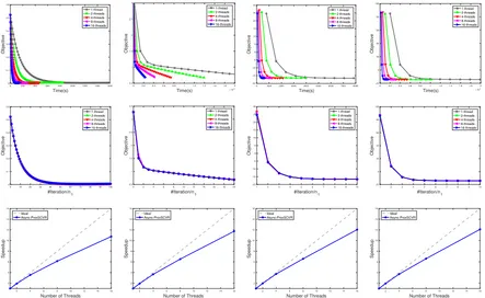
Figure 1: Results of the speedup experiment. Columns, from left to right, are the results on MDPs (100 states, 3 actions), MDPs (400 states, 10 actions), mean-variance problem (N=2000,d=300) and mean-variance problem (N=5000,d=300). The top row shows the curve of objective w.r.t the running time. The middle row shows the curve of objective w.r.t the number of iterations. The bottom row represents the time speedup with varying threads, where gray line represents ideal linear speedup.

policy π, rs,s1 is the immediate reward from s tos1, and

||w||1is the regularization term for sparsity. As mentioned

in (Wang, Liu, and Tang 2017), the objective function can be reformulated as the composition optimization problem (1) in which:

Gpwq “`wTϕp1q, qπ1pwq,¨ ¨ ¨, wTϕpSq, qπSpwq ˘

, (19)

Fppx1, y1,¨ ¨ ¨ , xS, ySqq “ S ÿ

s“1

pxs´ysq2. (20)

Following (Wang, Liu, and Tang 2017; Dann, Neumann, and Peters 2014), our experiments are conducted on random MDPs. In our first experiment, the MDP instance contains 100 states, and 3 actions at each state. The transition prob-abilities and rewards for each transition are uniformly sam-pling form [0, 1]. The sum of transition probabilities is then normalized to one. In our second experiment, the MDP in-stance contains 400 states, and 10 actions at each state. The transition probabilities and rewards are similarly sampling as in the first experiment. For both two experiments, we set regularization parameter γ “ 10´5, the discounted factor

λ “ 0.95. These are well-known examples to test the off-policy convergent algorithms (Geist and Scherrer 2014).

Application to Sparse Mean-variance Optimization

For the high-dimensional sparse portfolio management problem, the goal is to create a portfolio that have maximum

expected return but minimal variance of return. Specifically, givendassets, lettriuNi“1ĂRdbe the reward vectors at

dif-ferent time points, the objective function can be formulated as the following sparse mean-variance optimization:

x˚

“arg min

xPRdr

1

N N ÿ

i“1

pxri, xy ´

1

N N ÿ

j“1

xrj, xyq2

´ 1

N N ÿ

i“1

xri, xy `λ||x||1s, (21)

wherexP Rd denotes the investment quantity indassets.

Following (Huo, Gu, and Huang 2018; Yu and Huang 2017), the problem (21) is in the form of problem (1) in which:

Gjpxq “ px,´xrj, xyqT, xPRd, (22)

Fippx, yqq “ pxri, xy `yq2´ xri, xy, xPRd, yPR. (23)

In the experiment, we set N P t2000,5000u, d “ 300,

m “ 30 and the regularization parameterγ “ 10´5_{. The}

reward vectors are generated through Gaussian distributions with zero mean and positive semi-definite co-variance ma-trixΣ“LT_L_{, where}_L

PRdˆmandmăd. Each element ofLis drawn from the normal distribution.

(7)

0 100 200 300 400 500 600 700 800 900 1000 Time(s)

0 0.1 0.2 0.3 0.4 0.5 0.6

Objective

Async-ProxSCVR ASC-PG HOGWILD! Async-ProxSVRG com-SVR-ADMM

0 0.5 1 1.5 2 2.5 3 3.5 4

Time(s) 104

0.5 1 1.5 2 2.5 3 3.5

Objective

0 0.2 0.4 0.6 0.8 1 1.2 1.4 1.6 1.8 2

Time(s) 104

0 200 400 600 800 1000 1200

Objective

0 0.5 1 1.5 2 2.5

Time(s) 104

0 200 400 600 800 1000 1200

Objective

0 20 40 60 80 100 120 140 160 180 200 Time(s)

0 0.1 0.2 0.3 0.4 0.5 0.6

Objective

0 1000 2000 3000 4000 5000 6000 Time(s)

0.5 1 1.5 2 2.5 3 3.5

Objective

0 500 1000 1500 2000 2500 3000

Time(s)

0 200 400 600 800 1000 1200

Objective

0 500 1000 1500 2000 2500 3000 3500 4000 4500 5000

Time(s)

0 200 400 600 800 1000 1200

Objective

0 10 20 30 40 50 60 70 80 90 100 Time(s)

0 0.1 0.2 0.3 0.4 0.5 0.6

Objective

0 500 1000 1500 2000 2500 3000

Time(s)

0.5 1 1.5 2 2.5 3 3.5

Objective

0 200 400 600 800 1000 1200 1400 1600 1800 2000

Time(s) 0

200 400 600 800 1000 1200

Objective

0 200 400 600 800 1000 1200 1400 1600 1800 2000

Time(s) 0

200 400 600 800 1000 1200

Objective

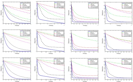
Figure 2: Comparison of five compared methods: HOGWILD!, Async-ProxSVRG, ASC-PG, com-SVR-ADMM and our pro-posed Async-ProxSCVR. As in Figure 1, columns, from left to right, are the results on MDPs (100 states, 3 actions), MDPs (400 states, 10 actions), mean-variance problem (N=2000,d=300) and mean-variance problem (N=5000,d=300). The rows from top to bottom represent the results on 1, 8, and 16 threads, respectively.

et al. 2011),Async-ProxSVRG(Meng et al. 2017), ASC-PG (Wang, Liu, and Tang 2017), com-SVR-ADMM (Yu and Huang 2017) and the proposedAsync-ProxSCVR.

Experimental Setting. For a fair comparison, we use the best tuned learning rates for compared methods, specifically, we select them from t100_,₁₀´1_,₁₀´2_,₁₀´3_,₁₀´4_,₁₀´5_u.

For variance reduction based algorithms, we set the inner loop sizem“kn1, in whichkis best tuned fromt0.5,1,2u.

The mini-batch sizes ofA,BandIare chosen casually as in (Huo, Gu, and Huang 2018). Furthermore, all of the meth-ods are coded in C++ using the standard thread library. We conduct all the experiments on an identical server which has 16 Intel(R) Xeon(R) E5-2650 CPUs and 64GB memory.

Experimental Results

Scaling with Number of Threads. In Figure 1, we show the speedup results of Async-ProxSCVR with varying num-ber of threads. The top line are results of objective function value with respect to running time. We observe that when we use more threads, the objective curve decreases faster. The middle line represents results of objective function value with respect to the number of iterations. The figures show that objective curves with different threads are almost coin-cident. It means that the negative effect of using stale iter-ation vector for calculating the gradient estimator vanishes to some extent. The bottom line shows results of the

run-ning time speedup. We can observe that the algorithm has a strong scaling when we use multiple threads. For instance, our proposed algorithm can achieve about 12ˆspeedup on 16 threads. Besides, results show that when the number of threads increases, our method has a nearly linear speedup in all experiments. These findings in the experiment are com-patible with our theoretical analysis.

Comparison with Other Methods. To demonstrate the superiority of our proposed Async-ProxSCVR, we conduct comparison experiments with all baseline methods. Figure 2 presents the objective curves versus the running time on 1, 8 and 16 threads, respectively. Results show that our proposed algorithm Async-ProxSCVR achieves fast empirical conver-gence rate compared with other benchmark algorithms in all four experiments. Furthermore, we see that our proposed al-gorithm is more robust to increasing threads.

Conclusion

In this paper, we introduce an asynchronous parallel method Async-ProxSCVR for problem (1) with nonsmooth reg-ularization penalty. We prove that our proposed Async-ProxSCVR can achieve a linear convergence rateOppn1` n2`κ3qlogp1{qqfor strongly convex case and a sublinear

convergence rate Oppn1`n2q 2

3_{_qfor general nonconvex

(8)

two representative composition optimization problems are conducted to demonstrate our convergence analysis.

Acknowledgments

This work is supported by the Zhejiang Provincial Natural Science Foundation (LR19F020005), National Natural Sci-ence Foundation of China (61572433, 61672125, 31471063, 61473259, 31671074) and thanks for a gift grant from Baidu inc. Also partially supported by the Hunan Provincial Science & Technology Project Foundation (2018TP1018, 2018RS3065) and the Fundamental Research Funds for the Central Universities.

References

Dann, C.; Neumann, G.; and Peters, J. 2014. Policy evalu-ation with temporal differences: A survey and comparison.

The Journal of Machine Learning Research15(1):809–883.

Defazio, A.; Bach, F.; and Lacoste-Julien, S. 2014. Saga: A fast incremental gradient method with support for non-strongly convex composite objectives. InAdvances in neural

information processing systems, 1646–1654.

Fang, C., and Lin, Z. 2017. Parallel asynchronous stochastic variance reduction for nonconvex optimization.

In Thirty-First AAAI Conference on Artificial Intelligence

(AAAI 2017), 794–800.

Friedman, J.; Hastie, T.; and Tibshirani, R. 2001. The

el-ements of statistical learning, volume 1. Springer series in

statistics New York, NY, USA:.

Geist, M., and Scherrer, B. 2014. Off-policy learning with eligibility traces: A survey. The Journal of Machine

Learn-ing Research15(1):289–333.

Hinton, G. E., and Roweis, S. T. 2003. Stochastic neighbor embedding. InAdvances in neural information processing

systems, 857–864.

Huo, Z., and Huang, H. 2017. Asynchronous mini-batch gradient descent with variance reduction for non-convex op-timization. In Thirty-First AAAI Conference on Artificial

Intelligence (AAAI 2017).

Huo, Z.; Gu, B.; and Huang, H. 2018. Accelerated method for stochastic composition optimization with nonsmooth regularization. In Thirty-Second AAAI Conference on

Ar-tificial Intelligence (AAAI 2018).

J. Reddi, S.; Sra, S.; Poczos, B.; and Smola, A. J. 2016. Proximal stochastic methods for nonsmooth nonconvex finite-sum optimization. InAdvances in neural information

processing systems, 1145–1153.

Johnson, R., and Zhang, T. 2013. Accelerating stochastic gradient descent using predictive variance reduction. In

Ad-vances in neural information processing systems, 315–323.

Lee, J. D.; Lin, Q.; Ma, T.; and Yang, T. 2015. Dis-tributed stochastic variance reduced gradient methods and a lower bound for communication complexity.arXiv preprint

arXiv:1507.07595.

Lian, X.; Wang, M.; and Liu, J. 2017. Finite-sum composi-tion optimizacomposi-tion via variance reduced gradient descent. In

The 20th International Conference on Artificial Intelligence

and Statistics.

Liu, J., and Wright, S. J. 2014. Asynchronous stochastic coordinate descent: Parallelism and convergence properties.

SIAM Journal on Optimization25(1).

Liu, J.; Wright, S. J.; R´e, C.; Bittorf, V.; and Sridhar, S. 2015. An asynchronous parallel stochastic coordinate de-scent algorithm.The Journal of Machine Learning Research

16(1):285–322.

Meng, Q.; Chen, W.; Yu, J.; Wang, T.; Ma, Z.; and Liu, T.-Y. 2017. Asynchronous stochastic proximal optimization algorithms with variance reduction. In Thirty-First AAAI

Conference on Artificial Intelligence (AAAI 2017).

Recht, B.; Re, C.; Wright, S.; and Niu, F. 2011. Hogwild: A lock-free approach to parallelizing stochastic gradient de-scent. In Advances in neural information processing sys-tems, 693–701.

Reddi, S. J.; Hefny, A.; Sra, S.; Poczos, B.; and Smola, A. J. 2015. On variance reduction in stochastic gradient descent and its asynchronous variants. InAdvances in neural

infor-mation processing systems, 2647–2655.

Reddi, S. J.; Hefny, A.; Sra, S.; Poczos, B.; and Smola, A. 2016. Stochastic variance reduction for nonconvex opti-mization. InInternational conference on machine learning, 314–323.

Schmidt, M.; Le Roux, N.; and Bach, F. 2017. Minimizing finite sums with the stochastic average gradient.

Mathemat-ical Programming162(1-2):83–112.

Shalev-Shwartz, S., and Zhang, T. 2013. Stochastic dual co-ordinate ascent methods for regularized loss minimization.

The Journal of Machine Learning Research14(2):567–599.

Shapiro, A.; Dentcheva, D.; and Ruszczy´nski, A. 2009.

Lectures on stochastic programming: modeling and theory.

SIAM.

Sutton, R. S., and Barto, A. G. 1998. Reinforcement

learn-ing: An introduction, volume 1. MIT press Cambridge.

Wang, M.; Fang, E. X.; and Liu, H. 2014. Stochastic compositional gradient descent: algorithms for minimizing compositions of expected-value functions. arXiv preprint

arXiv:1411.3803.

Wang, M.; Liu, J.; and Tang, E. X. 2017. Accelerating stochastic composition optimization. Journal of Machine

Learning Research18.

Xiao, L., and Zhang, T. 2014. A proximal stochastic gradient method with progressive variance reduction. SIAM Journal

on Optimization24(4):2057–2075.

Yu, Y., and Huang, L. 2017. Fast stochastic variance re-duced admm for stochastic composition optimization.arXiv

preprint arXiv:1705.04138.

Zhang, R., and Kwok, J. 2014. Asynchronous distributed admm for consensus optimization. InInternational