One-step ahead forecasting of geophysical processes within a purely statistical framework

(1)

RESEARCH LETTER

One-step ahead forecasting

of geophysical processes within a purely

statistical framework

Georgia Papacharalampous

*

_{, Hristos Tyralis and Demetris Koutsoyiannis}

Abstract

The simplest way to forecast geophysical processes, an engineering problem with a widely recognized challenging character, is the so-called “univariate time series forecasting” that can be implemented using stochastic or machine learning regression models within a purely statistical framework. Regression models are in general fast-implemented, in contrast to the computationally intensive Global Circulation Models, which constitute the most frequently used alternative for precipitation and temperature forecasting. For their simplicity and easy applicability, the former have been proposed as benchmarks for the latter by forecasting scientists. Herein, we assess the one-step ahead forecast-ing performance of 20 univariate time series forecastforecast-ing methods, when applied to a large number of geophysical and simulated time series of 91 values. We use two real-world annual datasets, a dataset composed by 112 time series of precipitation and another composed by 185 time series of temperature, as well as their respective standardized datasets, to conduct several real-world experiments. We further conduct large-scale experiments using 12 simulated datasets. These datasets contain 24,000 time series in total, which are simulated using stochastic models from the families of AutoRegressive Moving Average and AutoRegressive Fractionally Integrated Moving Average. We use the first 50, 60, 70, 80 and 90 data points for model-fitting and model-validation, and make predictions corresponding to the 51st, 61st, 71st, 81st and 91st respectively. The total number of forecasts produced herein is 2,177,520, among which 47,520 are obtained using the real-world datasets. The assessment is based on eight error metrics and accuracy statistics. The simulation experiments reveal the most and least accurate methods for long-term forecasting applica-tions, also suggesting that the simple methods may be competitive in specific cases. Regarding the results of the real-world experiments using the original (standardized) time series, the minimum and maximum medians of the absolute errors are found to be 68 mm (0.55) and 189 mm (1.42) respectively for precipitation, and 0.23 °C (0.33) and 1.10 °C (1.46) respectively for temperature. Since there is an absence of relevant information in the literature, the numerical results obtained using the standardized real-world datasets could be used as rough benchmarks for the one-step ahead predictability of annual precipitation and temperature.

Keywords: ARFIMA, Benchmarking time series forecasts, Machine learning, Neural networks, Precipitation, Random forests, Simple exponential smoothing, Support vector machines, Temperature, Univariate time series forecasting

© The Author(s) 2018. This article is distributed under the terms of the Creative Commons Attribution 4.0 International License (http://creativecommons.org/licenses/by/4.0/), which permits unrestricted use, distribution, and reproduction in any medium, provided you give appropriate credit to the original author(s) and the source, provide a link to the Creative Commons license, and indicate if changes were made.

Background

Forecasting geophysical variables in various time scales and horizons is useful in technological applica-tions (e.g. Giunta et al. 2015), but a difficult task as well.

Precipitation and temperature forecasting is mostly based on deterministic models as the Global Circulation Models (GCMs), which simulate the Earth’s atmosphere using numerical equations; therefore, deviating from tra-ditional time series forecasting, i.e. univariate time series forecasting. This particular deviation has been ques-tioned by forecasting scientists (Green and Armstrong 2007; Green et al. 2009; Fildes and Kourentzes 2011, see also the comments in Keenlyside 2011; McSharry 2011).

Open Access

*Correspondence: [email protected]

(2)

Traditional time series forecasting can be performed using several classes of regression models, as reviewed in De Gooijer and Hyndman (2006), while the two major classes are stochastic and machine learning. Regression models are in general fast-implemented in contrast to their computationally intensive alternative in precipita-tion and temperature forecasting, i.e. the GCMs. For their simplicity and easy applicability, the former have been proposed as benchmarks for the latter by Green et al. (2009).

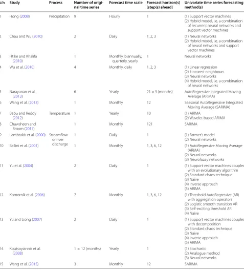
Recognizing the necessity of introducing traditional forecasting methods in temperature and precipitation forecasting, Armstrong and Fildes (2006) have recom-mended a relevant issue in one of the Journals special-ized in forecasting. Since then and despite the fact that considerable parts of books in hydrology are devoted to such methods (Sivakumar 2017, pp 63–145; Remesan and Mathew 2015, pp 71–110), there has not been a sys-tematic approach to the subject. However, studies adopt-ing statistical forecastadopt-ing approaches in geoscience are sporadically published in a variety of Journals. Within a statistical framework, Tyralis and Koutsoyiannis (2014, 2017) use Bayesian techniques for probabilistic climate forecasts under the established assumption of long-range dependence of the observed time series. In the latter study information from GCMs is used to improve the performance of the time series forecasting methods. Moreover, Table 1 presents some examples of studies using univariate time series forecasting approaches that do not utilize exogenous predictor variables to forecast precipitation or temperature variables, and streamflow or river discharge variables. The former can be considered as climatic or meteorological variables depending on the time scale of interest, while the latter can be considered as the results of precipitation (and other) variables and are more frequently modelled by describing this depend-ence using either deterministic or statistical methods. Such statistical approaches to modelling hydrological variables can be found in Chen et al. (2015), Gholami et al. (2015) and Taormina and Chau (2015).

In a somehow different direction, Papacharalampous et al. (2017c) conduct a multiple-case study, i.e. a syn-thesis of 50 single-case studies, by using monthly pre-cipitation and temperature time series of various lengths observed in Greece. Some important points regard-ing the comparison of univariate time series forecast-ing methods and additional concerns introduced when implementing the machine learning ones (hyperparam-eter optimization and lagged variable selection) in one- and multi-step ahead forecasting are illustrated in the latter study. Nevertheless, only large-scale forecast-pro-ducing studies could provide empirical solutions to sev-eral problems appearing in the field of (geophysical) time

series forecasting. Such studies are rare in the literature. Beyond geoscience, Makridakis and Hibon (2000) use a real-world dataset composed by 3003 time series, mainly originating from the business, industry, macroeconomic and microeconomic sectors, to assess the one- and multi-step ahead forecasting accuracy of 24 univariate time series forecasting methods. In geoscience, on the other hand, there are only four recent studies, all companions of the present, to be subsequently discussed.

Papacharalampous et al. (2017a) compare 11 stochastic and nine machine learning univariate time series fore-casting methods in multi-step ahead forefore-casting of geo-physical processes and (empirically) prove that stochastic and machine learning methods can perform equally well. The comparisons are conducted using 24,000 simulated time series of 110 values, 24,000 simulated time series of 310 values and 92 mean monthly time series of stream-flow with varying lengths, as well as 18 metrics. These 20 methods are also found to collectively compose a representative sample set, i.e. exhibiting a variety of forecasting performances with respect to the different metrics. Alongside with this study, Papacharalampous et al. (2017b) investigate the error evolution in multi-step ahead forecasting when adopting this specific set of methods. The tests are performed on 6000 simulated time series of 150 values, 6000 simulated time series of 350 values and the streamflow dataset used in Papacha-ralampous et al. (2017a). Some different behaviours are revealed within these experiments, also suggesting the fact that one- and multi-step ahead forecasting are dif-ferent problems to be examined for the same methods. Moreover, Tyralis and Papacharalampous (2017) focus on random forests, a well-known machine learning algo-rithm, with the aim to improve its one-step ahead fore-casting performance by conducting experiments on 16,000 simulated and 135 annual temperature time series of 101 values. Finally, Papacharalampous et al. (2018) investigate the multi-step ahead predictability of monthly precipitation and temperature by applying seven auto-matic univariate time series forecasting methods to a sample of 1552 monthly precipitation and 985 monthly temperature time series of 480 values.

(3)

time series of 91 values. These experiments complement the real-world ones by allowing the examination of a large variety of process behaviours, while they are also controlled to some extent, facilitating generalizations and increasing the understanding on the examined prob-lem. The number of forecasts produced using these real-world and simulated datasets are 47,520 and 2,130,000,

respectively, i.e. the largest among its companion studies. Our aim is twofold, to provide generalized results regard-ing one-step ahead forecastregard-ing within a purely statisti-cal framework [justified, for example, in Hyndman and Athanasopoulos (2013)] in geoscience and hopefully to establish the results obtained by the examination of the standardized real-world datasets as rough benchmarks Table 1 Examples of univariate time series forecasting in geoscience

s/n Study Process Number of

origi-nal time series Forecast time scale Forecast horizon(s) [step(s) ahead] Univariate time series forecasting method(s)

1 Hong (2008) Precipitation 9 Hourly 1 (1) Support vector machines

(2) Hybrid model, i.e. a combination of recurrent neural networks and support vector machines

2 Chau and Wu (2010) 2 Daily 1, 2, 3 (1) Neural networks

(2) Hybrid model, i.e. a combination of neural networks and support vector machines

3 Htike and Khalifa

(2010) 1 Monthly, biannually, quarterly, yearly 1 Neural networks

4 Wu et al. (2010) 4 Monthly, daily 1, 2, 3 (1) Linear regression

(2) k-nearest neighbours (3) Neural networks

(4) Hybrid model, i.e. a combination of neural networks

5 Narayanan et al.

(2013) 6 Yearly 21 × 3 (months) AutoRegressive Integrated Moving Average (ARIMA)

6 Wang et al. (2013) 1 Monthly 12 Seasonal AutoRegressive Integrated

Moving Average (SARIMA) 7 Babu and Reddy

(2012) Temperature 1 Yearly 10 (1) ARIMA(2) Wavelet-based ARIMA

8 Chawsheen and

Broom (2017) 1 Monthly 121 SARIMA

9 Lambrakis et al. (2000) Streamflow or river discharge

1 Daily 1 (1) Farmer’s model

(2) Neural networks

10 Ballini et al. (2001) 1 Monthly 1, 3, 6, 12 (1) AutoRegressive Moving Average

(ARMA) (2) Neural networks (3) Neurofuzzy networks

11 Yu et al. (2004) 2 Daily 1 (1) Support vector machines coupled

with an evolutionary algorithm (2) Standard chaos technique (3) Naïve

(4) Inverse approach (5) ARIMA

12 Komorník et al. (2006) 7 Monthly 1, 3, 6, 12 (1) Threshold AutoRegressive (AR)

with aggregation operators (2) Logistic smooth transition AR (3) Self-exciting threshold AR (4) Naïve

13 Yu and Liong (2007) 2 Daily 1 (1) Support vector machines coupled

with decomposition (2) Standard chaos technique (3) Naïve

(4) Inverse approach (5) ARIMA 14 Koutsoyiannis et al.

(2008) 1 × 12 (months) Yearly 1 (1) Stochastic(2) Analogue method

(3) Neural networks

(4)

for the one-step ahead predictability of annual precipita-tion and temperature. The establishment of forecasting benchmarks is meaningful, especially for the one-step ahead attempts, as the latter constitute the most simple ones and their accuracy can be quantified using a single metric, i.e. the absolute error.

Data and methods

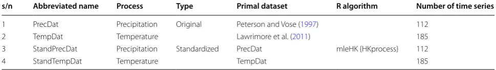
We use the datasets briefly described in Tables 2 and 3. The PrecDat and TempDat datasets are annual and originate from two larger monthly datasets, available in Peterson and Vose (1997) and Lawrimore et al. (2011) respectively. The sample period is from 1910 to 2000, so the following two conditions are simultaneously met: (1) there are no missing values, (2) the number of stations around the globe is the largest possible. We note that for sample periods extending after 2000 the number of retained stations would decrease rapidly. Figure 1 pre-sents the maps of the retained stations. The precipitation ones create a sufficiently dense network in the United States of America and in Scandinavia, while the retained temperature stations in the United States of America, in Japan and in a part of South Korea. As it is apparent from Table 2, the StandPrecDat and StandTempDat datasets simply contain the standardized time series of PrecDat and TempDat respectively.

Figure 1 also presents the histograms of the Hurst parameter maximum likelihood estimates (Tyralis and Koutsoyiannis 2011) of the formed real-world time series. These estimates are of importance within this study for two reasons: (1) we implement a univariate time series forecasting method (see later on in this section) that takes advantage of this information under the established assumption of long-range dependence, (2) we standard-ize the original real-world time series using the mean and standard deviation maximum likelihood estimates (estimated simultaneously with the Hurst parameter) of the Hurst–Kolmogorov process. The standard deviation estimates would be considerably different if we mod-elled the time series using independent normal variables (Tyralis and Koutsoyiannis 2011). For consistency pur-poses with respect to the real-world datasets of the pre-sent study (but also to approximate the typical length of annual geophysical time series), the simulated time series are of 91 values as well. They originate from the families of AutoRegressive Moving Average (ARMA(p,q)) and AutoRegressive Fractionally Integrated Moving Aver-age (ARFIMA(p,d,q)), the definitions of which can eas-ily be found in the literature, for example in Wei (2006), pp 6–65, 489–494. The simulations are performed with mean 0 and standard deviation of 1. Hereafter, to spec-ify a used R algorithm, we state its name accompanied Table 2 Datasets of this study (part 1): real-world datasets

s/n Abbreviated name Process Type Primal dataset R algorithm Number of time series

1 PrecDat Precipitation Original Peterson and Vose (1997) 112

2 TempDat Temperature Lawrimore et al. (2011) 185

3 StandPrecDat Precipitation Standardized PrecDat mleHK {HKprocess} 112

4 StandTempDat Temperature TempDat 185

Table 3 Datasets of this study (part 2): simulated datasets

s/n Abbreviated name Process Parameter(s) R algorithm Number of time series

5 SimDat_1 AR(1) φ₁= 0.7 arima.sim {stats} 2000

6 SimDat_2 AR(1) φ₁=−0.7

7 SimDat_3 AR(2) φ₁= 0.7, φ2= 0.2

8 SimDat_4 MA(1) θ₁= 0.7

9 SimDat_5 MA(1) θ₁=−0.7

10 SimDat_6 ARMA(1,1) φ₁= 0.7, θ₁= 0.7

11 SimDat_7 ARMA(1,1) φ₁=−0.7, θ1=−0.7

12 SimDat_8 ARFIMA(0,0.30,0) fracdiff.sim {fracdiff }

13 SimDat_9 ARFIMA(1,0.30,0) φ₁= 0.7

14 SimDat_10 ARFIMA(0,0.30,1) θ₁=−0.7

15 SimDat_11 ARFIMA(1,0.30,1) φ₁= 0.7, θ1=−0.7

(5)

(6)

by the name of the R package, denoted with {}. All algo-rithms are used with predefined values, unless specified differently.

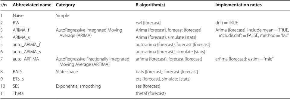
We implement the forecasting methods described in Tables 4, 5 and 6. The latter constitute an adapted repro-duction from Papacharalampous et al. (2017a). Naïve is the last observation benchmark, while random walk (RW) is a commonly used variation of Naïve (Hyndman and Athanasopoulos 2013). Regarding the AutoRegres-sive Integrated Moving Average (ARIMA) methods, the ARIMA_f and auto_ARIMA_f forecasting models use the same algorithm with the ARIMA_s and auto_ARIMA_s simulation models respectively, although the innovations are set to be zero in the former ones. The latter applies to the auto_ARFIMA method as well, which is com-monly used for modelling processes that are assumed to exhibit long-range dependence. These five methods esti-mate the involved parameters using the maximum likeli-hood method. BATS, ETS and SES stand for Box-Cox transformation, ARMA errors, Trend and Seasonal com-ponents (De Livera et al. 2011); Error, Trend and Season-ality (or ExponenTial Smoothing); and Simple Exponential Smoothing respectively. Further information about the latter models can be found in Hyndman and Athanaso-poulos (2013), while Theta is introduced in Assimakopou-los and NikolopouAssimakopou-los (2000). All the stochastic methods use procedures like those presented in Hyndman and Khandakar (2008). The machine learning methods, on the other hand, are based on a somehow different algorith-mic approach. This fact is easily perceivable through the alongside examination of Tables 4, 5 and 6.

The assessment of the one-step ahead forecasting per-formance is based on the error metrics and accuracy sta-tistics of Table 7.

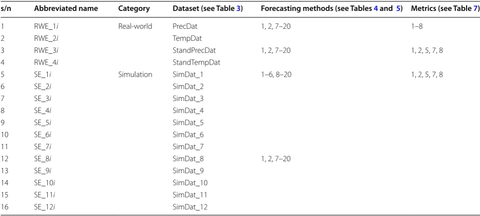
We conduct the experiments described in Tables 8 and 9. We use each dataset in five experiments; every time

examining different parts of the time series according to Table 9. While the application of the stochastic meth-ods does not require a validation set (since all the model parameters are estimated using other procedures, such as the maximum likelihood estimation), the same does not apply to the application of the machine learning methods (except NN_3). For each of the latter, we fit the candidate models defined in Table 5 to the fitting set, i.e. the first 33, 40, 47, 53 or 60 values, and subsequently use them to make predictions corresponding to the validation set, i.e. the next 17, 20, 23, 27 or 30 values respectively. Finally, we decide on the “optimal” model, i.e. the one exhibiting the smallest root mean square error on the validation set. We fit this model to the first 50, 60, 70, 80 or 90 values and make predictions corresponding to the 51st, 61st, 71st, 81st or 91st value respectively.

The only assumption of our methodological approach concerns the application of the auto_ARFIMA method within the real-world experiments and is that the annual precipitation and temperature variables can be suf-ficiently modelled by the normal distribution. This assumption is rather reasonable (implied by the Central Limit Theorem; Koutsoyiannis 2008, chapter 2.5.6) and could hardly harm the results. In general, such funda-mental assumptions are preferable to the introduction of extra parameters, e.g. to using the Box-Cox transforma-tion to normalize the data. The rest of the methods are non-parametric and, thus, not affected by the possible non-normality. To take advantage of some well-known theoretical properties, in the SE_1i–SE_7i simulation experiments the ARIMA_f and ARIMA_s methods are given the same AutoRegressive (AR) and Moving Aver-age (MA) orders used in the respective simulation pro-cess, while d is set 0. These two methods, as well as the simple, auto_ARIMA_f, auto_ARIMA_s and auto_ ARFIMA methods serve as reference points within our

Table 4 Univariate time series forecasting methods of this study (part 1): stochastic methods

s/n Abbreviated name Category R algorithm(s) Implementation notes

1 Naïve Simple

2 RW rwf {forecast} drift = TRUE

3 ARIMA_f AutoRegressive Integrated Moving

Average (ARIMA) Arima {forecast}, forecast {forecast} Arima {forecast}: include.mean include.drift = FALSE, method == TRUE, ”ML”

4 ARIMA_s Arima {forecast}, simulate {stats}

5 auto_ARIMA_f auto.arima {forecast}, forecast {forecast}

6 auto_ARIMA_s auto.arima {forecast}, simulate {stats}

7 auto_ARFIMA AutoRegressive Fractionally Integrated

Moving Average (ARFIMA) arfima {forecast}, forecast {forecast} arfima {forecast}: estim = ”mle”

8 BATS State space bats {forecast}, forecast {forecast}

9 ETS_s ets {forecast}, simulate {stats}

10 SES Exponential smoothing ses {forecast}

(7)

Table

5

Univ

aria

te time series f

or

ec

asting methods of

this study (par

t 2): machine learning methods

s/n A bbr evia ted name C at egor y M odel struc tur e inf orma tion R algorithm(s) Implemen ta tion not es H yperpar amet er optimiz ed using g rid sear ch (g rid v alues) Lagged v ariable selec tion pr oc e-dur e (see T able 6 ) 12 NN_1 Neural net w or ks

Single hidden la

yer multila yer per ceptr on CasesS er ies {r

miner}, fit {r

miner},

lfor

ecast {r

miner}, nnet {nnet}

Number of hidden nodes (0, 1, …, 15)

1 13 NN_2 2 14 NN_3 nnetar {f or ecast} 3 15 RF_1 Random f or ests Br eiman

’s random f

or

ests algo

-rithm with 500 g

ro wn tr ees CasesS er ies {r

miner}, fit {r

miner}, lfor ecast {r miner}, randomF or est {randomF or est}

Number of var

iables randomly

sampled as candidat

es at each

split (1, …, 5)

1 16 RF_2 2 17 RF_3 3 18 SVM_1 Suppor t v ec tor machines

Radial basis k

er nel “G aussian ” func tion, C = 1, epsilon = 0.1 CasesS er ies {r

miner}, fit {r

miner},

lfor

ecast {r

miner}, ksvm {k

er nlab} Sig ma in verse k er nel width (2 n, n = − 8, −

7, …, 6)

(8)

approach. In particular, ARIMA_f, auto_ARIMA_f and auto_ARFIMA are theoretically expected to be the most accurate within our simulation experiments [for an expla-nation see Papacharalampous et al. (2017a), chapter 2], while BATS is also expected to perform well in these experiments, since it comprises an ARMA model. In summary, the experiments are controlled to some extent, while their components (datasets, methods and metrics)

are selected to provide a multifaceted approach to the problem of one-step ahead forecasting in geoscience.

Results and discussion

In this section, we summarize the basic quantitative and qualitative information gained from the experiments of the present study, while the total amount is available in the Additional files 1, 2, 3, 4, 5, 6 and 7. We further Table 6 Lagged variable selection procedures adopted for the machine learning methods of Table 5

s/n Time lags R algorithm

1 The corresponding to an estimated value for the AutoCorrelation Function (ACF) acf {stats}

2 The corresponding to a statistical important estimated value for the ACF. If there is no statistical important estimated value for the

ACF, the corresponding to the largest estimated value acf {stats}

3 According to nnetar {forecast}, i.e. the time lags 1, …, n, where n is the number of AutoRegressive (AR) parameters that are fitted to

the time series data ar {stats}

Table 7 Error metrics and accuracy statistics of this study

s/n Abbreviated name Full name Category Values Optimum value

1 E Error Error metrics (−∞, +∞) 0

2 AE Absolute error [0, +∞) 0

3 PE Percentage error (−∞, +∞) 0

4 APE Absolute percentage error [0, +∞) 0

5 MdoAE Median of the absolute errors Accuracy statistics [0, +∞) 0

6 MdoAPE Median of the absolute percentage errors [0, +∞) 0

7 LRC Linear regression coefficient (−∞, +∞) 1

8 R2 Coefficient of determination [0, 1] 1

Table 8 Experiments of this study

The symbol i can take the values stated in Table 9

s/n Abbreviated name Category Dataset (see Table 3) Forecasting methods (see Tables 4 and 5) Metrics (see Table 7)

1 RWE_1i Real-world PrecDat 1, 2, 7–20 1–8

2 RWE_2i TempDat

3 RWE_3i StandPrecDat 1, 2, 7–20 1, 2, 5, 7, 8

4 RWE_4i StandTempDat

5 SE_1i Simulation SimDat_1 1–6, 8–20 1, 2, 5, 7, 8

6 SE_2i SimDat_2

7 SE_3i SimDat_3

8 SE_4i SimDat_4

9 SE_5i SimDat_5

10 SE_6i SimDat_6

11 SE_7i SimDat_7

12 SE_8i SimDat_8 1, 2, 7–20

13 SE_9i SimDat_9

14 SE_10i SimDat_10

15 SE_11i SimDat_11

(9)

discuss the findings and explicate their contribution in light of the literature.

Experiments using the precipitation datasets

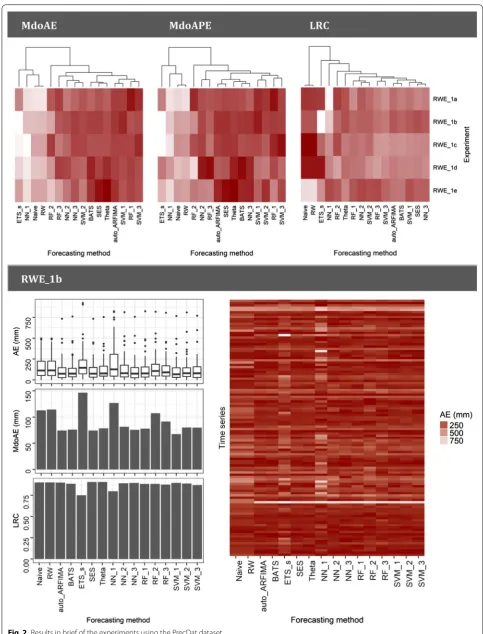
For the experiments using the PrecDat dataset, the mini-mum AE value is 0 (practically) and the maximini-mum around 1,750 mm (for forecasts produced by the simple forecast-ing methods, i.e. Naïve and RW), while the respective values for the APE error metric are 0 (practically) and 1.64 (for a forecast produced by NN_1). The MdoAE and MdoAPE values are summarized in Tables 10 and 11 respectively. The minimum MdoAE is 68 mm, while the maximum is 189 mm. These two values are in the same order of magnitude as the smallest and average standard

deviation estimates of the time series respectively. The minimum MdoAPE value is 0.09 and the maximum 0.22, while the respective LRC values are 0.73 and 1.18. The best LRC value (1.00) is measured within RWE_1c for the simple forecasting methods, while the best R2 value (0.84) is measured within RWE_1d for BATS. The worst LRC and R2 values are 0.73 for RF_2 within RWE_1d and 0.54 for NN_1 within RWE_1a respectively.

In Fig. 2 we present a graphical summary of the experi-ments using the PrecDat dataset. The values in the three upper heatmaps are scaled in the row direction and the darker the colour within a specific row the bet-ter the forecasts. In fact, heatmaps are used in this study instead of conventional tables, since they allow the easy extract of qualitative information. The relative perfor-mance of the forecasting methods differs to some degree across the various RWE_1i experiments, with ETS_s and NN_1 being the worst performing in terms of MdoAE and MdoAPE, followed by the simple methods. On the other hand, in terms of LRC Naïve and RW exhibit rather the best overall performance. In the downer heatmap of Fig. 2 we zoom into the RWE_1b experiment. By its examination we observe that all the implemented fore-casting methods can perform well or bad, depending on the individual case. This fact is also apparent in the side-by-side boxplots of Fig. 2. Furthermore, we observe that for one specific time series the AE values measured are very high for all the forecasts apart from those produced by the simple forecasting methods.

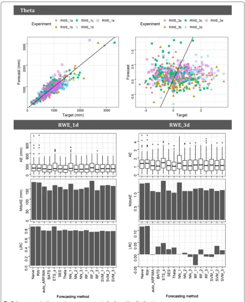
Regarding the experiments using the StandPrec-Dat dataset, the minimum AE value is 0 and the maxi-mum around 10. The MdoAE values are summarized in Table 12. The minimum MdoAE is 0.55, while the maxi-mum is 1.42. These two values are 45% smaller and 42% larger than 1 (standard deviation of the standardized time series) respectively. Since there is an absence of rel-evant information in the literature, these values could be used as rough benchmarks for the predictability of annual precipitation. Most preferably, a representative sample set of univariate time series forecasting meth-ods could be implemented at least for benchmarking purposes alongside with any other forecasting attempt. Moreover, the minimum and maximum LRC values are −0.25 and 0.25 respectively, the former measured for ETS_s and the latter for RW. Finally, the minimum R2 value is 0 (practically), while the maximum is 0.09, meas-ured within SE_3a for ETS_s. In addition to this numeri-cal information, Fig. 3 presents a brief comparison between the experiments using the PrecDat and Stand-PrecDat datasets. As illustrated in this figure, the relative performance of the forecasting methods with respect to AE and MdoAE in the experiments using the latter data-set is mostly similar to the one in the experiments using Table 9 Part of the time series used within each

experi-ment according to the i value

s/n i Data points of each time series

used for the model-fitting (required for all models) and model-validation (required for the machine learning models)

Data points of each time series used for model-testing

1 a 1, 2, 3, …, 50 51

2 b 1, 2, 3, …, 60 61

3 c 1, 2, 3, …, 70 71

4 d 1, 2, 3, …, 80 81

5 e 1, 2, 3, …, 90 91

Table 10 Minimum, maximum and mean values of the MdoAE within the experiments using the PrecDat dataset

The minimum of the minimum values and the maximum of the maximum values are in italic

Minimum (mm) Maximum (mm) Mean (mm)

RWE_1a 111 (RF_1) 172 (NN_1) 135

RWE_1b 68 (SVM_1) 146 (ETS_s) 91

RWE_1c 91 (SVM_3) 171 (ETS_s) 119

RWE_1d 143 (BATS) 189 (RF_2) 162

RWE_1e 98 (Theta) 150 (NN_1) 122

Table 11 Minimum, maximum and mean values of the MdoAPE within the experiments using the PrecDat dataset

Minimum Maximum Mean

RWE_1a 0.12 (RF_1) 0.21 (RW) 0.16

RWE_1b 0.09 (SVM_1) 0.18 (ETS_s) 0.12

RWE_1c 0.12 (SVM_3) 0.21 (NN_1) 0.15

RWE_1d 0.15 (BATS) 0.22 (NN_1) 0.17

(10)

(11)

the former dataset. Nevertheless, the LRC (and R2) val-ues are far worse when using the standardized datasets. In fact, standardization results to processes with different predictability with respect to the original.

Experiments using the temperature datasets

In Fig. 4 we present a graphical summary of the experi-ments using the TempDat dataset. For these experiexperi-ments the minimum AE value is 0 and the maximum around 43 °C (for a forecast produced by NN_2), while the respective APE values are 0 and 9.64 (for a forecast pro-duced by ETS_s). The MdoAE and MdoAPE values are summarized in Tables 13 and 14 respectively. The mini-mum MdoAE is 0.23 °C, while the maximini-mum is 1.10 °C. These two values are in the same order of magnitude as the smallest and largest standard deviation estimates of the temperature time series respectively. The respective values for MdoAPE are 0.02 and 0.08. The minimum LRC value is 0.95 and the maximum is 1.02; all the LRC val-ues are close to the optimum. Finally, the minimum R2 value is 0.78, measured for NN_2 within RWE_2b, while all the rest R2 values are higher than 0.97 with maximum 1 (practically), measured for the auto_ARFIMA method within RWE_2b. In summary, the relative performance of the forecasting methods varies across the different experiments conducted using the TempDat dataset. The auto_ARFIMA, BATS, SES, Theta and NN_3 seem to be well performing in terms of MdoAE and MdoAPE when applied to these temperature time series compared to the overall picture, while the simple methods are far the best in terms of MdoAE within the RWE_2d experiment. ETS_s and NN_1 are the worst performing within all the experiments apart from RWE_2c, in which the simple methods exhibit the worst performance. Finally, by com-paring the numerical results of the experiments using the PrecDat and TempDat dataset, we observe the fact that temperature is more predictable than precipitation.

Regarding the experiments using the StandTempDat, the minimum AE value is 0 and the maximum around 18.91. The MdoAE values are summarized in Table 15.

The minimum MdoAE value is 0.33, while the maximum is 1.46. These two values are 67% smaller and 46% larger than 1 (standard deviation of the standardized time series) respectively and could be used as rough bench-marks for the predictability of annual temperature (for an explanation see the subsection entitled “Experiments

using the precipitation datasets”). The minimum LRC

value is 0.04 and the maximum is 0.76, the former meas-ured for SVM_1 and the latter for RW. Finally, the mini-mum R2 value is 0.03, while the maximini-mum is 0.48. The latter value is measured for Naïve in RWE_4a. Figure 5 facilitates a comparison between the experiments using the TempDat and StandTempDat datasets. Here as well, we observe that the relative performance of the fore-casting methods with respect to AE and MdoAE in the experiments using the standardized precipitation time series mostly does not vary from the respective relative performance when using the original temperature time series. We further note that the LRC (and R2) values are worse when using the standardized temperature dataset, while they are better for the latter than for the standard-ized precipitation dataset.

Experiments using the simulated datasets

The subsequently reported information constitutes the provided empirical solution to the problem of one-step ahead forecasting in geoscience. Nonetheless, this solution is rather qualitative than quantitative (although the results are also stated quantitatively), since the respective experi-ments use unscaled data that could be assumed as real-world data in a standardized form (such as StandPrecDat and StandTempDat) with different predictability than the original (for example, see the subsections entitled “ Experi-ments using the precipitation datasets” and “Experiments using the temperature datasets”). In fact, the experiments using standardized precipitation and temperature can facilitate a connection between the experiments using the same data in their original form and the experiments using the simulated datasets. A graphical summary of the latter experiments is available in Fig. 6.

The generalized findings of the present study are the following:

(1) The E values are approximately symmetric around 0

(mean value of the simulations).

(2) The results may vary significantly across the simula-tion experiments using different simulated datasets and across the different time series within a specific experiment depending on the forecasting method. (3) Consequently, the relative performance of the

fore-casting methods may also vary significantly across the simulation experiments using different simulated datasets.

Table 12 Minimum, maximum and mean values of the MdoAE within the experiments using the StandPrecDat dataset

RWE_3a 0.70 (RF_1) 1.22 (NN_1) 0.92

RWE_3b 0.55 (SVM_2) 0.95 (ETS_s) 0.69

RWE_3c 0.72 (BATS) 1.42 (NN_1) 0.86

RWE_3d 0.99 (Theta) 1.42 (ETS_s) 1.14

(12)

(13)

(14)

(4) On the contrary, the relative performance of the fore-casting methods is slightly affected by the length of the time series for the experiments of the present study. The same has been found to mostly apply to the multi-step ahead forecasting performance of the

same methods in Papacharalampous et al. (2017a) for

two other time series lengths.

(5) Some forecasting methods are more accurate than others. The best-performing methods are ARIMA_f, auto_ARIMA_f, auto_ARFIMA, BATS, SES and Theta. This good performance of the former four methods when applied to ARMA and ARFIMA processes is expected from theory, while the Theta

forecasting method has also performed well in the

M3-Competition (Makridakis and Hibon 2000) and

is expected to have a similar performance with SES

(Hyndman and Billah 2003). The five

above-men-tioned forecasting methods are all stochastic.

(6) All the machine learning methods except for NN_1 (mostly NN_3 and SVM_3) are comparable to the best-performing methods, as it has also been found to apply in the experiments of Papacharalampous

et al. (2017a, b). Likewise, in Tyralis and

Papacha-ralampous (2017), random forests are competitive

with the ARFIMA and Theta benchmarks.

(7) The simple methods are competitive in specific simu-lation experiments, as suggested for specific cases in

Cheng et al. (2017), Makridakis and Hibon (2000)

and Papacharalampous et al. (2017a) as well.

Never-theless, they also stand out because of their bad per-formance in other simulation experiments.

(8) Most of the far outliers are produced by neural net-works.

The minimum AE value for the forecasts is 0 (prac-tically) and the maximum around 155 (produced by NN_2). The MdoAE values are summarized in Tables 16 and 17. Especially, the latter is useful in supporting Observations (5–7). The minimum MdoAE is 0.65, while the maximum is 2.91. These two values are 35% smaller and 191% larger than 1 (standard deviation of the simula-tions) respectively. Furthermore, in spite of Observation (4), the MdoAE values may decrease on the level of the second or even the first decimal, when moving from the simulation experiments using time series of 51 values to those of 91 values, with the NN_1 forecasting method exhibiting the largest improvement. The minimum LRC value is −0.88 and the maximum is 0.94, both measured for RW, while the minimum and maximum values pro-duced by Naïve differ in the second and third decimal respectively. This range holds a complete interpretation of the observed within the real-world experiments varia-tions in the performance of the simple methods in terms of LRC from extremely good to extremely bad (with respect to the overall picture). Finally, the minimum R2 value is 0 (practically), measured for ETS_s within several experiments, while the maximum is 0.84 within SE_9b for Naïve.

Conclusions

The simulation experiments reveal the most and least accurate methods for long-term one-step ahead fore-casting applications, also suggesting that the simple methods may be competitive in specific cases. Further-more, the relative performance of the forecasting meth-ods is slightly affected by the time series length for the Table 13 Minimum, maximum and mean values of the

MdoAE within the experiments using the TempDat dataset

Minimum (°C) Maximum (°C) Mean (°C)

RWE_2a 0.42 (NN_3) 0.72 (NN_1) 0.51

RWE_2b 0.23 (Theta) 0.54 (NN_1) 0.32

RWE_2c 0.38 (BATS) 0.66 (RW) 0.47

RWE_2d 0.78 (RW) 1.10 (NN_3) 1.01

RWE_2e 0.38 (Theta) 0.62 (ETS_s) 0.46

Table 14 Minimum, maximum and mean values of the MdoAPE within the experiments using the TempDat data-set

RWE_2a 0.04 (Theta) 0.06 (NN_1) 0.04

RWE_2b 0.02 (auto_ARFIMA) 0.05 (ETS_s) 0.03

RWE_2c 0.03 (SVM_1) 0.06 (RW) 0.04

RWE_2d 0.07 (Naïve) 0.08 (NN_1) 0.08

RWE_2e 0.03 (RF_1) 0.05 (NN_1) 0.04

Table 15 Minimum, maximum and mean values of the MdoAE within the experiments using the StandTempDat dataset

RWE_4a 0.61 (BATS) 0.93 (ETS_s) 0.71

RWE_4b 0.33 (Theta) 0.73 (NN_1) 0.47

RWE_4c 0.56 (SES) 0.96 (ETS_s) 0.69

RWE_4d 1.20 (NN_1) 1.46 (Theta) 1.36

(15)

simulation experiments of this study (using time series of 51, 61, 71, 81, 91 values), while it strongly depends on the process. Also importantly, the experiments using the original real-world time series result to minimum and

maximum medians of the absolute errors of 68 and 189 mm for precipitation, and 0.23 and 1.10 °C for tempera-ture respectively. Additionally, the experiments using the standardized real-world time series suggest that the

(16)

(17)

minimum and maximum medians of the absolute errors are 0.55 and 1.42 for precipitation, and 0.33 and 1.46 for temperature respectively. These latter numerical results could be used as a rough upper boundary for the

one-step ahead predictability of annual precipitation and temperature.

We subsequently state the limitations of this study and some future directions. The provided empirical solution to the problem of one-step ahead forecasting in geosci-ence is rather qualitative than quantitative, while the experiments using standardized precipitation and tem-perature data have offered rough benchmarks only. In the future more real-world data could be used to develop improved benchmarks for assessing the respective pre-dictabilities. It would be of interest to further investigate how these predictabilities depend on the location from which the data originate. In this case, more stations span-ning around the globe would be required. Moreover, a direct and large-scale comparison, set on a common base (if this is feasible), between deterministic and statistical approaches to forecasting geophysical processes would be useful and interesting. Another limitation of this study is related to the adopted modelling approach, i.e. the data-driven one, according to which the selection of the model does not depend on the properties of the examined pro-cess and, therefore, the latter are mostly not investigated. Furthermore, the improvement of the performance of the machine learning models requires extensive comparisons between different procedures of hyperparameter opti-mization and lagged variable selection. Finally, future research could focus on the examination of the respective predictabilities, when using exogenous predictor vari-ables as well, while a definitely worth-stated future direc-tion is related to the adopdirec-tion of probabilistic forecasting methods, instead of the point forecasting ones.

Abbreviations

ACF: AutoCorrelation Function; AR: AutoRegressive; ARFIMA: AutoRegressive Fractionally Integrated Moving Average; ARIMA: AutoRegressive Integrated Moving Average; ARMA: AutoRegressive Moving Average; MA: Moving Aver-age; SARIMA: Seasonal AutoRegressive Integrated Moving Average.

Authors’ contributions

GP and HT worked on the analyses equally and to all of their aspects. GP, HT and DK discussed the results and contributed in the writing of the main manuscript. All authors read and approved the final manuscript.

Additional files

Additional file 1. Exploration of the datasets.

Additional file 2. Experiments using the PrecDat dataset.

Additional file 3. Experiments using the TempDat dataset.

Additional file 4. Experiments using the StandPrecDat dataset.

Additional file 5. Experiments using the StandTempDat dataset.

Additional file 6. Experiments using the simulated datasets, part 1.

Additional file 7. Experiments using the simulated datasets, part 2. Table 16 Minimum, maximum and mean values of the

MdoAE within the simulation experiments

Table 17 Minimum, maximum and mean values of the MdoAE for each method within the simulation experi-ments

Naïve 0.68 (SE_3c) 2.88 (SE_7a) 1.12

RW 0.69 (SE_9c) 2.91 (SE_7e) 1.13

ARIMA_f 0.65 (SE_3c) 0.72 (SE_7a) 0.69

ARIMA_s 0.91 (SE_2a) 1.04 (SE_3a) 0.96

auto_ARIMA_f 0.66 (SE_7d) 0.75 (SE_6c) 0.70

auto_ARIMA_s 0.91 (SE_4c) 1.02 (SE_3d) 0.97

auto_ARFIMA 0.67 (SE_10e) 0.73 (SE_10d) 0.69

BATS 0.67 (SE_3c) 0.76 (SE_6c) 0.71

ETS_s 0.93 (SE_3d) 2.11 (SE_7e) 1.14

SES 0.66 (SE_3c) 1.52 (SE_7e) 0.83

Theta 0.66 (SE_3c) 1.57 (SE_7a) 0.84

NN_1 0.90 (SE_7e) 1.16 (SE_7a) 1.01

NN_2 0.72 (SE_8c) 0.89 (SE_5b) 0.79

NN_3 0.69 (SE_8c) 0.84 (SE_6c) 0.74

RF_1 0.71 (SE_8c) 1.08 (SE_6a) 0.82

RF_2 0.72 (SE_8c) 1.04 (SE_6c) 0.83

RF_3 0.72 (SE_3c) 0.98 (SE_6c) 0.80

SVM_1 0.71 (SE_8e) 1.23 (SE_7a) 0.86

SVM_2 0.68 (SE_8c) 1.01 (SE_7a) 0.81

(18)

Acknowledgements

We thank the Editor Bellie Sivakumar and two anonymous reviewers, whose comments have substantially improved the quality of this paper.

The analyses and visualizations have been performed in R Programming Language (R Core Team 2017) by using the contributed R packages forecast (Hyndman and Khandakar 2008, Hyndman et al. 2017), fracdiff (Fraley et al.

2012), gdata (Warnes et al. 2017), ggplot2 (Wickham 2016), HKprocess (Tyralis

2016), kernlab (Karatzoglou et al. 2004), knitr (Xie 2014, 2015, 2017), nnet (Venables and Ripley 2002), randomForest (Liaw and Wiener 2002), readr (Wickham et al. 2017) and rminer (Cortez 2010, 2016).

We acknowledge the Asia Oceania Geoscience Society (AOGS) for provid-ing the publication cost. A preliminary research by Papacharalampous et al.

(2017d) was presented in the 14th AOGS Annual Meeting.

Competing interests

The authors declare that they have no competing interests.

Availability of data and materials

This is a fully reproducible research paper; all the codes and data, as well as their outcome results, are available in the Additional files (Papacharalampous and Tyralis 2018). The sources of the real-world datasets are Lawrimore et al. (2011) and Peterson and Vose (1997).

Funding

This research has not received any funding.

Publisher’s Note

Springer Nature remains neutral with regard to jurisdictional claims in pub-lished maps and institutional affiliations.

Received: 31 August 2017 Accepted: 17 March 2018

References

Armstrong JS, Fildes R (2006) Making progress in forecasting. Int J Forecast 22(3):433–441. https://doi.org/10.1016/j.ijforecast.2006.04.007

Assimakopoulos V, Nikolopoulos K (2000) The theta model: a decomposi-tion approach to forecasting. Int J Forecast 16(4):521–530. https://doi. org/10.1016/S0169-2070(00)00066-2

Babu CN, Reddy BE (2012) Predictive data mining on average global tempera-ture using variants of ARIMA models. In: Proceeding of 2012 international conference on advances in engineering, science and management (ICAESM)

Ballini R, Soares S, Andrade MG (2001) Multi-step-ahead monthly streamflow forecasting by a neurofuzzy network model. In: IFSA World Congress and 20th NAFIPS International Conference, pp 992–997. https://doi. org/10.1109/nafips.2001.944740

Chau KW, Wu CL (2010) A hybrid model coupled with singular spectrum analy-sis for daily rainfall prediction. J Hydroinform 12(4):458–473. https://doi. org/10.2166/hydro.2010.032

Chawsheen TA, Broom M (2017) Seasonal time-series modeling and forecast-ing of monthly mean temperature for decision makforecast-ing in the Kurdistan Region of Iraq. J Stat Theory Pract 11(4):604–633. https://doi.org/10.1080/ 15598608.2017.1292484

Chen XY, Chau KW, Busari AO (2015) A comparative study of population-based optimization algorithms for downstream river flow forecasting by a hybrid neural network model. Eng Appl Artif Intell 46(Part A):258–268.

https://doi.org/10.1016/j.engappai.2015.09.010

Cheng KS, Lien YT, Wu YC, Su YF (2017) On the criteria of model performance evaluation for real-time flood forecasting. Stoch Environ Res Risk Assess 31(5):1123–1146. https://doi.org/10.1007/s00477-016-1322-7

Cortez P (2010) Data mining with neural networks and support vector machines using the R/rminer tool. In: Perner P (ed) Advances in data mining. Applications and theoretical aspects. Springer, Heidelberg, pp 572–583. https://doi.org/10.1007/978-3-642-14400-4_44

Cortez P (2016) rminer: data mining classification and regression methods. R package version 1.4.2. https://CRAN.R-project.org/package=rminer

De Gooijer JG, Hyndman RJ (2006) 25 years of time series forecasting. Int J Forecast 22(3):443–473. https://doi.org/10.1016/j.ijforecast.2006.01.001

De Livera AM, Hyndman RJ, Snyder RS (2011) Forecasting time series with complex seasonal patterns using exponential smoothing. J Am Stat Assoc 106(496):1513–1527. https://doi.org/10.1198/jasa.2011.tm09771

Fildes R, Kourentzes N (2011) Validation and forecasting accuracy in models of climate change. Int J Forecast 27(4):968–995. https://doi.org/10.1016/j. ijforecast.2011.03.008

Fraley C, Leisch F, Maechler M, Reisen V, Lemonte A (2012) fracdiff: fractionally differenced ARIMA aka ARFIMA(p,d,q) models. R package version 1.4-2.

https://CRAN.R-project.org/package=fracdiff

Gholami V, Chau KW, Fadaee F, Torkaman J, Ghaffari A (2015) Modeling of groundwater level fluctuations using dendrochronology in alluvial aquifers. J Hydrol 529(Part 3):1060–1069. https://doi.org/10.1016/j. jhydrol.2015.09.028

Giunta G, Salerno R, Ceppi A, Ercolani G, Mancini M (2015) Benchmark analysis of forecasted seasonal temperature over different climatic areas. Geosci Lett 2:9. https://doi.org/10.1186/s40562-015-0026-z

Green KC, Armstrong JS (2007) Global warming: forecasts by scientists versus scientific forecasts. Energy Environ 18(7):997–1021. https://doi. org/10.1260/095830507782616887

Green KC, Armstrong JS, Soon W (2009) Validity of climate change forecasting for public policy decision making. Int J Forecast 25(4):826–832. https:// doi.org/10.1016/j.ijforecast.2009.05.011

Hong WC (2008) Rainfall forecasting by technological machine learning models. Appl Math Comput 200(1):41–57. https://doi.org/10.1016/j. amc.2007.10.046

Htike KK, Khalifa OO (2010) Rainfall forecasting models using focused time-delay neural networks. In: Proceeding of 2010 international conference on computer and communication engineering (ICCCE). https://doi. org/10.1109/iccce.2010.5556806

Hyndman RJ, Athanasopoulos G (2013) Forecasting: principles and practice. OTexts: Melbourne, Australia. http://otexts.org/fpp/

Hyndman RJ, Billah B (2003) Unmasking the Theta method. Int J Forecasting 19(2):287–290. https://doi.org/10.1016/S0169-2070(01)00143-1

Hyndman RJ, Khandakar Y (2008) Automatic time series forecasting: the forecast package for R. J Stat Softw 27(3):1–22. https://doi.org/10.18637/ jss.v027.i03

Hyndman RJ, O’Hara-Wild M, Bergmeir C, Razbash S, Wang E (2017) forecast: forecasting functions for time series and linear models. R package version 8.2. https://CRAN.R-project.org/package=forecast

Karatzoglou A, Smola A, Hornik K, Zeileis A (2004) kernlab—an S4 package for kernel methods in R. J Stat Softw 11(9):1–20

Keenlyside NS (2011) Commentary on “Validation and forecasting accuracy in models of climate change”. Int J Forecast 27(4):1000–1003. https://doi. org/10.1016/j.ijforecast.2011.07.002

Komorník J, Komorníková M, Mesiar R, Szökeová D, Szolgay J (2006) Com-parison of forecasting performance of nonlinear models of hydrological time series. Phys Chem Earth Parts A/B/C 31(18):1127–1145. https://doi. org/10.1016/j.pce.2006.05.006

Koutsoyiannis D (2008) Probability and statistics for geophysical processes. National Technical University of Athens, Athens. https://doi.org/10.13140/ RG.2.1.2300.1849/1

Koutsoyiannis D, Yao H, Georgakakos A (2008) Medium-range flow predic-tion for the Nile: a comparison of stochastic and deterministic methods. Hydrol Sci J 53(1):142–164. https://doi.org/10.1623/hysj.53.1.142

Lambrakis N, Andreou AS, Polydoropoulos P, Georgopoulos E, Bountis T (2000) Nonlinear analysis and forecasting of a brackish karstic spring. Water Resour Res 36(4):875–884. https://doi.org/10.1029/1999WR900353

Lawrimore JH, Menne MJ, Gleason BE, Williams CN, Wuertz DB, Vose RS, Ren-nie J (2011) An overview of the Global Historical Climatology Network monthly mean temperature data set, version 3. J Geophys Res. https:// doi.org/10.1029/2011JD016187

Liaw A, Wiener M (2002) Classification and regression by randomForest. R News 2(3):18–22

(19)

McSharry PE (2011) Validation and forecasting accuracy in models of climate change: comments. Int J Forecast 27(4):996–999. https://doi. org/10.1016/j.ijforecast.2011.07.003

Narayanan P, Basistha A, Sarkar S, Kamna S (2013) Trend analysis and ARIMA modelling of pre-monsoon rainfall data for western India. C R Geosci 345(1):22–27. https://doi.org/10.1016/j.crte.2012.12.001

Papacharalampous GA, Tyralis H (2018) One-step ahead forecasting of geo-physical processes within a purely statistical framework: supplementary material. figshare. https://doi.org/10.6084/m9.figshare.5357359.v1

Papacharalampous GA, Tyralis H, Koutsoyiannis D (2017a) Comparison of stochastic and machine learning methods for the multi-step ahead forecasting of hydrological processes. Preprints. https://doi.org/10.20944/ preprints201710.0133.v1

Papacharalampous GA, Tyralis H, Koutsoyiannis D (2017b) Error evolution in multi-step ahead streamflow forecasting for the operation of hydropower reservoirs. Preprints. https://doi.org/10.20944/preprints201710.0129.v1

Papacharalampous GA, Tyralis H, Koutsoyiannis D (2017c) Forecasting of geophysical processes using stochastic and machine learning algorithms. Eur Water 59:161–168

Papacharalampous GA, Tyralis H, Koutsoyiannis D (2017d) Large scale simula-tion experiments for the assessment of one-step ahead forecasting prop-erties of stochastic and machine learning point estimation methods. Asia Oceania Geosciences Society (AOGS) 14th Annual Meeting, Singapore.

http://www.itia.ntua.gr/en/docinfo/1719/

Papacharalampous GA, Tyralis H, Koutsoyiannis D (2018) Predictability of monthly temperature and precipitation using automatic time series forecasting methods. Acta Geophys. https://doi.org/10.1007/ s11600-018-0120-7

Peterson TC, Vose RS (1997) An Overview of the Global Historical Climatol-ogy Network temperature database. B Am Meteorol Soc. 78:2837–2849.

https://doi.org/10.1175/1520-0477(1997)078<2837:AOOTGH>2.0.CO;2

R Core Team (2017) R: a language and environment for statistical computing. R Foundation for Statistical Computing, Vienna

Remesan R, Mathew J (2015) Hydrological data driven model-ling. Springer International Publishing, New York. https://doi. org/10.1007/978-3-319-09235-5

Sivakumar B (2017) Chaos in hydrology: bridging determinism and stochastic-ity. Springer, New York. https://doi.org/10.1007/978-90-481-2552-4

Taormina R, Chau KW (2015) Data-driven input variable selection for rainfall– runoff modeling using binary-coded particle swarm optimization and extreme learning machines. J Hydrol 529(Part 3):1617–1632. https://doi. org/10.1016/j.jhydrol.2015.08.022

Tyralis H (2016) HKprocess: Hurst–Kolmogorov process. R package version

0.0-2. https://CRAN.R-project.org/package=HKprocess

Tyralis H, Koutsoyiannis D (2011) Simultaneous estimation of the parameters of the Hurst–Kolmogorov stochastic process. Stoch Environ Res Risk Assess 25(1):21–33. https://doi.org/10.1007/s00477-010-0408-x

Tyralis H, Koutsoyiannis D (2014) A Bayesian statistical model for deriving the predictive distribution of hydroclimatic variables. Clim Dyn 42(11– 12):2867–2883. https://doi.org/10.1007/s00382-013-1804-y

Tyralis H, Koutsoyiannis D (2017) On the prediction of persistent processes using the output of deterministic models. Hydrol Sci J 62(13):2083–2102 Tyralis H, Papacharalampous G (2017) Variable selection in time series

forecast-ing usforecast-ing random forests. Algorithms 10(4):114. https://doi.org/10.3390/ a10040114

Venables WN, Ripley BD (2002) Modern applied statistics with S, 4th edn. Springer-Verlag, New York. https://doi.org/10.1007/978-0-387-21706-2

Wang S, Feng J, Liu G (2013) Application of seasonal time series model in the precipitation forecast. Math Comput Model 58(3–4):677–683. https://doi. org/10.1016/j.mcm.2011.10.034

Wang W, Chau K, Xu D, Chen XY (2015) Improving forecasting accuracy of annual runoff time series using ARIMA based on EEMD decomposi-tion. Water Resour Manag 29(8):2655–2675. https://doi.org/10.1007/ s11269-015-0962-6

Warnes GR, Bolker B, Gorjanc G, Grothendieck G, Korosec A, Lumley T, Mac-Queen D, Magnusson A, Rogers J et al (2017) gdata: various R program-ming tools for data manipulation. R package version 2.18.0. https://

CRAN.R-project.org/package=gdata

Wei WWS (2006) Time series analysis, univariate and multivariate methods, 2nd edn. Pearson Addison Wesley, Boston

Wickham H (2016) ggplot2: elegant graphics for data analysis, 2nd edn. Springer International Publishing, Cham. https://doi. org/10.1007/978-3-319-24277-4

Wickham H, Hester J, Francois R, Jylänki J, Jørgensen M (2017) readr: read rectangular text data. R package version 1.1.1. https://CRAN.R-project.

org/package=readr

Wu CL, Chau KW, Fan C (2010) Prediction of rainfall time series using modular artificial neural networks coupled with data-preprocessing techniques. J Hydrol 389(1–2):146–167. https://doi.org/10.1016/j.jhydrol.2010.05.040

Xie Y (2014) knitr: a comprehensive tool for reproducible research in R. In: Stodden V, Leisch F, Peng RD (eds) Implementing reproducible computa-tional research. Chapman and Hall/CRC, Boca Raton

Xie Y (2015) Dynamic documents with R and knitr, 2nd edn. Chapman and Hall/CRC, Boca Raton

Xie Y (2017) knitr: a general-purpose package for dynamic report generation in R. R package version 1.17. https://CRAN.R-project.org/package=knitr

Yu X, Liong SY (2007) Forecasting of hydrologic time series with ridge regression in feature space. J Hydrol 332(3–4):290–302. https://doi. org/10.1016/j.jhydrol.2006.07.003