Sparse Boosting

Sparse Boosting

Peter B ¨uhlmann [email protected]

Seminar f¨ur Statistik ETH Z¨urich

Z¨urich, CH-8092, Switzerland

Bin Yu [email protected]

Department of Statistics University of California Berkeley, CA 94720-3860, USA

Editors: Yoram Singer and Larry Wasserman

Abstract

We propose Sparse Boosting (the SparseL2Boost algorithm), a variant on boosting with the squared error loss. SparseL2Boost yields sparser solutions than the previously proposed L2Boosting by minimizing some penalized L2-loss functions, the FPE model selection criteria, through small-step gradient descent. Although boosting may give already relatively sparse solutions, for example corresponding to the soft-thresholding estimator in orthogonal linear models, there is sometimes a desire for more sparseness to increase prediction accuracy and ability for better variable selection: such goals can be achieved with SparseL2Boost.

We prove an equivalence of SparseL2Boost to Breiman’s nonnegative garrote estimator for orthogonal linear models and demonstrate the generic nature of SparseL2Boost for nonparametric interaction modeling. For an automatic selection of the tuning parameter in SparseL2Boost we propose to employ the gMDL model selection criterion which can also be used for early stopping of L2Boosting. Consequently, we can select between SparseL2Boost and L2Boosting by comparing their gMDL scores.

Keywords: lasso, minimum description length (MDL), model selection, nonnegative garrote, regression

1. Introduction

Since its inception in a practical form in Freund and Schapire (1996), boosting has obtained and maintained its outstanding performance in numerous empirical studies both in the machine learning and statistics literatures. The gradient descent view of boosting as articulated in Breiman (1998, 1999), Friedman et al. (2000) and R¨atsch et al. (2001) provides a springboard for the understanding of boosting to leap forward and at the same time serves as the base for new variants of boosting to be generated. In particular, the L2Boosting (Friedman, 2001) takes the simple form of refitting a base learner to residuals of the previous iteration. It coincides with Tukey’s (1977) twicing at its second iteration and reproduces matching pursuit of Mallat and Zhang (1993) when applied to a dictionary or collection of fixed basis functions. A somewhat different approach has been suggested by R¨atsch

et al. (2002). B¨uhlmann and Yu (2003) investigated L2Boosting for linear base procedures (weak

special case calculation implies that the resistance to the over-fitting behavior of boosting could be due to the fact that the complexity of boosting increases at an extremely slow pace.

Recently Efron et al. (2004) made an intriguing connection for linear models between L2Boosting

and Lasso (Tibshirani, 1996) which is anℓ1_{-penalized least squares method. They consider a}

modi-fication of L2Boosting, called forward stagewise least squares (FSLR) and they show that for some special cases, FSLR with infinitesimally small step-sizes produces a set of solutions which coincides with the set of Lasso solutions when varying the regularization parameter in Lasso. Furthermore, Efron et al. (2004) proposed the least angle regression (LARS) algorithm whose variants give a clever computational short-cut for FSLR and Lasso.

For high-dimensional linear regression (or classification) problems with many ineffective pre-dictor variables, the Lasso estimate can be very poor in terms of prediction accuracy and as a variable selection method, see Meinshausen (2005). There is a need for more sparse solutions than

pro-duced by the Lasso. Our new SparseL2Boost algorithm achieves a higher degree of sparsity while

still being computationally feasible, in contrast to all subset selection in linear regression whose computational complexity would generally be exponential in the number of predictor variables.

For the special case of orthogonal linear models, we prove here an equivalence of SparseL2Boost

to Breiman’s (1995) nonnegative garrote estimator. This demonstrates the increased sparsity of SparseL2Boost over L2Boosting which is equivalent to soft-thresholding (due to Efron et al. (2004) and Theorem 2 in this article).

Unlike Lasso or the nonnegative garrote estimator, which are restricted to a (generalized) linear

model or basis expansion using a fixed dictionary, SparseL2Boost enjoys much more generic

appli-cability while still being computationally feasible in high-dimensional problems and yielding more sparse solutions than boosting orℓ1_{-regularized versions thereof (see R¨atsch et al., 2002; Lugosi and} Vayatis, 2004). In particular, we demonstrate its use in the context of nonparametric second-order interaction modeling with a base procedure (weak learner) using thin plate splines, improving upon Friedman’s (1991) MARS.

Since our SparseL2Boost is based on the final prediction error criterion, it opens up the possi-bility of bypassing the computationally intensive cross-validation by stopping early based on the model selection score. The gMDL model selection criterion (Hansen and Yu, 2001) uses a data-driven penalty to the L2-loss and as a consequence bridges between the two well-known AIC and BIC criteria. We use it in the SparseL2Boost algorithm and for early stopping of L2Boosting. Fur-thermore, we can select between SparseL2Boost and L2Boosting by comparing their gMDL scores.

2. Boosting with the Squared Error Loss

We assume that the data are realizations from

(X1,Y1), . . . ,(Xn,Yn),

where Xi∈Rp denotes a p-dimensional predictor variable and Yi ∈R a univariate response. In

the sequel, we denote by x(j) _{the jth component of a vector x∈R}p_{. We usually assume that the}

pairs(Xi,Yi)are i.i.d. or from a stationary process. The goal is to estimate the regression function F(x) =E[Y_|X =x]which is well known to be the (population) minimizer of the expected squared error lossE[(Y₋F(X))2_].

it-erations. The final boosted procedure takes the form of linear combinations of the base procedures. For L2Boosting, based on the squared error loss, one simply fits the base procedure to the original data to start with, then uses the residuals from the previous iteration as the new response vector and refits the base procedure, and so on. As we will see in section 2.2, L2Boosting is a “constrained” minimization of the empirical squared error risk n−1∑n_i=1(Yi−F(Xi))2(with respect to F(·)) which yields an estimator ˆF(_·). The regularization of the empirical risk minimization comes in implicitly by the choice of a base procedure and by algorithmical constraints such as early stopping or penalty barriers.

2.1 Base Procedures Which Do Variable Selection

To be more precise, a base procedure is in our setting a function estimator based on the data

{(Xi,Ui); i=1, . . . ,n}, where U1, . . . ,Un denote some (pseudo-) response variables which are not necessarily the original Y1, . . . ,Yn. We denote the base procedure function estimator by

ˆ

g(_·) =gˆ₍X,U)(·), (1)

where X= (X1, . . . ,Xn)and U= (U1, . . . ,Un).

Many base procedures involve some variable selection. That is, only some of the components of the p-dimensional predictor variables Xi are actually contributing in (1). In fact, almost all of the successful boosting algorithms in practice involve base procedures which do variable selection: examples include decision trees (see Freund and Schapire, 1996; Breiman, 1998; Friedman et al., 2000; Friedman, 2001), componentwise smoothing splines which involve selection of the best single predictor variable (see B¨uhlmann and Yu, 2003), or componentwise linear least squares in linear models with selection of the best single predictor variable (see Mallat and Zhang, 1993; B¨uhlmann, 2006).

It will be useful to represent the base procedure estimator (at the observed predictors Xi) as a hat-operator, mapping the (pseudo-) response to the fitted values:

H

: U_7→(gˆ(X,U)(X1), . . . ,gˆ(X,U)(Xn)),U= (U1, . . . ,Un).

If the base procedure selects from a set of predictor variables, we denote the selected predictor variable index by ˆ

S

_{⊂ {}1, . . . ,p_}, where ˆ

S

has been estimated from a specified setΓof subsets of variables. To emphasize this, we write for the hat operator of a base procedure

H

Sˆ : U7→(gˆ(X(Sˆ)_,U)(X1), . . . ,gˆ_(X(Sˆ)_,U)(Xn)),U= (U1, . . . ,Un), (2)

where the base procedure ˆg(X,U)(·) =gˆ_(X(Sˆ)_,U)(·)depends only on the components X(

ˆ

S)_{from X. The}

Componentwise linear least squares in linear model (see Mallat and Zhang, 1993; B¨uhlmann, 2006)

We select only single variables at a time fromΓ=_{1,2, . . . ,p_}. The selector ˆ

S

chooses the predictor variable which reduces the residual sum of squares most when using least squares fitting:

ˆ

S

=argmin_1≤j≤p n

∑

i=1

(Ui−ˆγjXi(j))2,γˆj= ∑ n

i=1UiXi(j)

∑n

i=1(X

(j)

i )2

(j=1, . . . ,p).

The base procedure is then

ˆ

g₍X,U)(x) =γˆSˆx( ˆ S)_,

and its hat operator is given by the matrix

H

_Sˆ =X(Sˆ)(X(Sˆ))T,X(j)= (X₁(j), . . . ,Xn(j))T.

L2Boosting with this base procedure yields a linear model with model selection and parameter

estimates which are shrunken towards zero. More details are given in sections 2.2 and 2.4.

Componentwise smoothing spline (see B¨uhlmann and Yu, 2003)

Similarly to a componentwise linear least squares fit, we select only one single variable at a time fromΓ=_{1,2, . . . ,p_}. The selector ˆ

S

chooses the predictor variable which reduces residual sum of squares most when using a smoothing spline fit. That is, for a given smoothing spline operator with fixed degrees of freedomd_.f_{.(which is the trace of the corresponding hat matrix)}

ˆ

S

=argmin_1≤j≤p n

∑

i=1

(Ui−gˆj(Xi(j)))2, ˆ

gj(·)is the fit from the smoothing spline to U versus X(j)withd.f.

Note that we use the same degrees of freedomd_.f_{.for all components j’s. The hat-matrix}

corre-sponding to ˆgj(·)is denoted by

H

j which is symmetric; the exact from is not of particular interest here but is well known, see Green and Silverman (1994). The base procedure is

ˆ

g₍X,U)(x) =gˆSˆ(x( ˆ S)_),

and its hat operator is then given by a matrix

H

_Sˆ. Boosting with this base procedure yields an

additive model fit based on selected variables (see B¨uhlmann and Yu, 2003).

Pairwise thin plate splines

Generalizing the componentwise smoothing spline, we select pairs of variables fromΓ=_{(j,k); 1_≤ j<k_≤p_}. The selector ˆ

S

chooses the two predictor variables which reduce residual sum of squares most when using thin plate splines with two arguments:

ˆ

S

=argmin_1≤j<k≤p n

∑

i=1

(Ui−gˆj,k(Xi(j),X

(k)

i ))2, ˆ

where the degrees of freedomd.f._{is the same for all components j}<_{k. The hat-matrix} correspond-ing to ˆgj,kis denoted by

H

j,k which is symmetric; again the exact from is not of particular interest but can be found in Green and Silverman (1994). The base procedure is

ˆ

g(X,U)(x) =gˆSˆ(x( ˆ S)_),

where x(Sˆ) denotes the 2-dimensional vector corresponding to the selected pair in ˆ

S

, and the hat operator is then given by a matrix

H

_Sˆ. Boosting with this base procedure yields a nonparametric fit with second order interactions based on selected pairs of variables; an illustration is given in section 3.4.

In all the examples above, the selector is given by

ˆ

S

=argminS_∈Γ n

∑

i=1

(Ui−(HSU)i)2 (3)

Also (small) regression trees can be cast into this framework. For example for stumps, Γ=

{(j,cj,k); j=1, . . . ,p,k=1, . . . ,n−1}, where cj,1< . . . <cj,n−1are the mid-points between (non-tied) observed values X_i(j)(i=1, . . . ,n). That is,Γdenotes here the set of selected single predictor variables and corresponding split-points. The parameter values for the two terminal nodes in the

stump are then given by ordinary least squares which implies a linear hat matrix

H

_(j,c

j,k). Note

however, that for mid-size or large regression trees, the optimization over the set Γis usually not

done exhaustively.

2.2 L2Boosting

Before introducing our new SparseL2Boost algorithm, we describe first its less sparse counterpart

L2Boosting, a boosting procedure based on the squared error loss which amounts to repeated fitting

of residuals with the base procedure ˆg(X,U)(·). Its derivation from a more general functional gradient

descent algorithm using the squared error loss has been described by many authors, see Friedman (2001).

L2Boosting

Step 1 (initialization). ˆF0(_·)_≡0 and set m=0.

Step 2. Increase m by 1.

Compute residuals Ui=Yi−Fˆm−1(Xi) (i=1, . . . ,n)and fit the base procedure to the current resid-uals. The fit is denoted by ˆfm(·) =gˆ(X,U)(·).

Update

ˆ

Fm(·) =Fˆm₋1(·) +νfˆm(·), where 0<ν_≤1 is a pre-specified step-size parameter.

With m=2 andν=1, L2Boosting has already been proposed by Tukey (1977) under the name “twicing”. The number of iterations is the main tuning parameter for L2Boosting. Empirical

ev-idence suggests that the choice for the step-sizeνis much less crucial as long as νis small; we

usually useν=0.1. The number of boosting iterations may be estimated by cross-validation. As an

alternative, we will develop in section 2.5 an approach which allows to use some model selection criteria to bypass cross-validation.

2.3 SparseL2Boost

As described above, L2Boosting proceeds in a greedy way: if in Step2 the base procedure is fitted

by least squares and when using ν=1, L2Boosting pursues the best reduction of residual sum of

squares in every iteration.

Alternatively, we may want to proceed such that the out-of-sample prediction error would be most reduced, that is we would like to fit a function ˆgX,U(from the class of weak learner estimates)

such that the out-of-sample prediction error becomes minimal. This is not exactly achievable since the out-sample prediction error is unknown. However, we can estimate it via a model selection criterion. To do so, we need a measure of complexity of boosting. Using the notation as in (2), the L2Boosting operator in iteration m is easily shown to be (see B¨uhlmann and Yu, 2003)

B

m=I−(I−ν

H

Sˆm)· ··· ·(I−ν

H

Sˆ1), (4)

where ˆ

S

_m denotes the selector in iteration m. Moreover, if all the

H

S are linear (that is the hat

matrix), as in all the examples given in section 2.1, L2Boosting has an approximately linear

rep-resentation, where only the data-driven selector ˆ

S

brings in some additional nonlinearity. Thus, in many situations (for example the examples in the previous section 2.1 and decision tree base pro-cedures), the boosting operator has a corresponding matrix-form when using in (4) the hat-matrices for

H

S. The degrees of freedom for boosting are then defined as

trace(Bm) =trace(I−(I−ν

H

Sˆm)···(I−ν

H

Sˆ1)).

This is a standard definition for degrees of freedom (see Green and Silverman, 1994) and it has been used in the context of boosting in B¨uhlmann (2006). An estimate for the prediction error of L2Boosting in iteration m can then be given in terms of the final prediction error criterion FPEγ

(Akaike, 1970):

n

∑

i=1

(Yi−Fˆm(Xi))2+γ·trace(

B

m). (5)

2.3.1 THESPARSEL2BOOSTALGORITHM

For SparseL2Boost, the penalized residual sum of squares in (5) becomes the criterion to move from

iteration m₋1 to iteration m. More precisely, for

B

a (boosting) operator, mapping the response

vector Y to the fitted variables, and a criterion C(RSS,k), we use the following objective function to boost:

T(Y,

B

) =C n

∑

i=1

(Yi−(BY)i)2,trace(B)

!

For example, the criterion could be FPEγfor someγ>0 which corresponds to

C_γ(RSS,k) =RSS+γ_·k. (7)

An alternative which does not require the specification of a parameter γas in (7) is advocated in

section 2.5.

The algorithm is then as follows.

SparseL2Boost

Step 1 (initialization). ˆF0(·)≡0 and set m=0. Step 2. Increase m by 1.

Search for the best selector

˜

S

_m=argmin_S∈ΓT(Y,trace(Bm(S))),

B

_m(S) =I₋(I₋

H

S)(I−ν

H

S˜m−1)···(I−ν

H

S˜1),

(for m=1:

B

₁(S) =

H

S).

Fit the residuals Ui=Yi−Fˆm−1(Xi)with the base procedure using the selected ˜

S

m which yields a function estimate

ˆ

fm(·) =gˆS˜m;(X,U)(·),

where ˆgS;(X,U)(·)corresponds to the hat operator

H

S from the base procedure. Step 3 (update). Update,

ˆ

Fm(·) =Fˆm−1(·) +νfˆm(·).

Step 4 (iteration). Repeat Steps 2 and 3 for a large number of iterations M.

Step 5 (stopping). Estimate the stopping iteration by

ˆ

m=argmin_1≤m≤MT(Y,trace(Bm)),

B

m=I−(I−ν

H

S˜m)···(I−ν

H

S˜1).

The final estimate is ˆFmˆ(·).

2.4 Connections to the Nonnegative Garrote Estimator

SparseL2Boost based on Cγ as in (7) enjoys a surprising equivalence to the nonnegative garrote

estimator (Breiman, 1995) in an orthogonal linear model. This special case allows explicit expres-sions to reveal clearly that SparseL2Boost (aka nonnegative-garrote) is sparser than L2Boosting (aka soft-thresholding).

Consider a linear model with n orthonormal predictor variables,

Yi= n

∑

j=1

βjx(ij)+εi, i=1, . . . ,n,

n

∑

i=1

x(_ij)x(_ik)=δjk, (8)

whereδjk denotes the Kronecker symbol, andε1, . . . ,εnare i.i.d. random variables with E[εi] =0 and Var(εi) =σ2_ε <∞. We assume here the predictor variables as fixed and non-random. Using the standard regression notation, we can re-write model (8) as

Y=Xβ+ε, XTX=XXT =I, (9)

with the n_×n design matrix X= (x(_ij))i,j=1,...,n, the parameter vectorβ= (β1, . . . ,βn)T, the response vector Y= (Y1, . . . ,Yn)T and the error vectorε= (ε1, . . . ,εn)T. The predictors could also be basis functions gj(ti)at observed values tiwith the property that they build an orthonormal system.

The nonnegative garrote estimator has been proposed by Breiman (1995) for a linear regression model to improve over subset selection. It shrinks each ordinary least squares (OLS) estimated coefficient by a nonnegative amount whose sum is subject to an upper bound constraint (the garrote). For a given response vector Y and a design matrix X (see (9)), the nonnegative garrote estimator takes the form

ˆ

βNngar,j=cjβˆOLS,j

such that

n

∑

i=1

(Yi−(X ˆβNngar)i)2is minimized, subject to cj≥0, p

∑

j=1

cj≤s, (10)

for some s>0. In the orthonormal case from (8), since the ordinary least squares estimator is

simply ˆβOLS,j= (XTY)j=Zj, the nonnegative garrote minimization problem becomes finding cj’s such that

n

∑

j=1

(Zj−cjZj)2is minimized, subject to cj≥0, n

∑

j=1 cj≤s.

Introducing a Lagrange multiplierτ>0 for the sum constraint gives the dual optimization problem: minimizing

n

∑

j=1

(Zj−cjZj)2+τ n

∑

j=1

This minimization problem has an explicit solution (Breiman, 1995):

cj= (1−λ/|Zj|2)+, λ=τ/2,

where u+=max(0,u). Hence ˆβNngar,j= (1−λ/|Zj|2)+Zjor equivalently,

ˆ

βNngar,j=



 

 

Zj−λ/|Zj|, if sign(Zj)Z2j ≥λ,

0, if Z2_j <λ,

Zj+λ/|Zj|, if sign(Zi)Z2j ≤ −λ.

, where Zj= (XTY)j. (12)

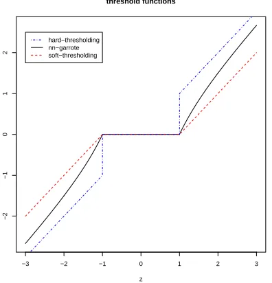
We show in Figure 1 the nonnegative garrote threshold function in comparison to hard- and soft-thresholding, the former corresponding to subset variable selection and the latter to the Lasso (Tib-shirani, 1996). Hard-thresholding either yields the value zero or the ordinary least squares estima-tor; the nonnegative garrote and soft-thresholding either yield the value zero or a shrunken ordinary least squares estimate, where the shrinkage towards zero is stronger for the soft-threshold than for the nonnegative garrote estimator. Therefore, for the same amount of “complexity” or “degrees of freedom” (which is in case of hard-thresholding the number of ordinary least squares estimated vari-ables), hard-thresholding (corresponding to subset selection) will typically select the fewest number of variables (non-zero coefficient estimates) while the nonnegative garrote will include more vari-ables and the soft-thresholding will be the least sparse in terms of the number of selected varivari-ables; the reason is that for the non-zero coefficient estimates, the shrinkage effect, which is slight in the nonnegative garotte and stronger for soft-thresholding, causes fewer degrees of freedom for every

−3 −2 −1 0 1 2 3

−2

−1

0

1

2

threshold functions

z hard−thresholding nn−garrote soft−thresholding

Figure 1: Threshold functions for subset selection or hard-thresholding (dashed-dotted line), non-negative garrote (solid line) and lasso or soft-thresholding (dashed line).

The following result shows the equivalence of the nonnegative garrote estimator and SparseL2Boost with componentwise linear least squares (using ˆm iterations) yielding coefficient estimates ˆβ(_SparseBoostmˆ) _,j. Theorem 1 Consider the model in (8) and any sequence(γn)n∈N. For SparseL₂Boost with

compo-nentwise linear least squares, based on Cγn as in (7) and using a step-sizeν, as described in section

2.3, we have

ˆ

β(mˆ)

SparseBoost,j=βˆNngar,jin (12) with parameterλn= 1

2γn(1+ej(ν)), max

1≤i≤n|ej(ν)| ≤ν/(1−ν)→0(ν→0).

A proof is given in section 5. Note that the sequence(γn)n∈Ncan be arbitrary and does not need

to depend on n (and likewise for the correspondingλn). For the orthogonal case, Theorem 1 yields

the interesting interpretation of SparseL2Boost as the nonnegative garrote estimator.

We also describe here for the orthogonal case the equivalence of L2Boosting with

component-wise linear least squares (yielding coefficient estimates ˆβ(_Boostm) _,j) to soft-thresholding. A closely re-lated result has been given in Efron et al. (2004) for the forward stagewise linear regression method which is similar to L2Boosting. However, our result is for (non-modified) L2Boosting and brings out more explicitly the role of the step-size.

The soft-threshold estimator for the unknown parameter vectorβ, is

ˆ

βso f t,j=



 

 

Zj−λ, if Zj≥λ,

0, if_|Zj|<λ, Zj+λ, if Zj≤ −λ.

where Zj= (XTY)j. (13)

Theorem 2 Consider the model in (8) and a thresholdλn in (13) for any sequence(λn)n∈N. For

L2Boosting with componentwise linear least squares and using a step-sizeν, as described in section 2.2, there exists a boosting iteration m, typically depending onλn,νand the data, such that

ˆ

β(m)

Boost,j=βˆso f t,jin (13) with threshold of the formλn(1+ej(ν)), where max

1≤j≤n|ej(ν)| ≤ν/(1−ν)→0(ν→0).

A proof is given in section 5. We emphasize that the sequence (λn)n∈N can be arbitrary: in

particular,λndoes not need to depend on sample size n.

2.5 The gMDL choice for the criterion function

The FPE criterion function C(_·,_·)in (7) requires in practice the choice of a parameterγ. In principle, we could tune this parameter using some cross-validation scheme. Alternatively, one could use a

parameter value corresponding to well-known model selection criteria such as AIC (γ=2) or BIC

(γ=log n). However, in general, the answer to whether to use AIC or BIC depends on the true

(with a shape hyperparameter) for the variance and conditioning on the variance, the linear model

parameterβfollows an independent multivariate normal prior with the given variance multiplied by

a scale hyperparameter. The two hyperparameters are then optimized based on the MDL principle and their coding costs are included in the code length. Because of the adaptive choices of the hyperparameters, the resulted gMDL criterion has a data-dependent penalty for each dimension, instead of the fixed penalty 2 or log n for AIC or BIC, respectively. In other words, gMDL bridges

the AIC and BIC criteria by having a data-dependent penalty log(F) as given below in (14). The

F in the gMDL penalty is related to the signal to noise ratio (SNR), as shown in Hansen and Yu (1999). Moreover, the gMDL criterion has an explicit analytical expression which depends only on the residual sum of squares and the model dimension or complexity. It is worth noting that we will not need to tune the criterion function as it will be explicitly given as a function of the data only. The gMDL criterion function takes the form

CgMDL(RSS,k) =log(S) + k

nlog(F),

S= RSS n₋k,F=

∑n

i=1Yi2−RSS

kS . (14)

Here, RSS denotes again the residual sum of squares as in formula (6) (first argument of the function C(_·,_·)).

In the SparseL2Boost algorithm in section 2.3.1, if we take T(Y,

B

) =CgMDL(RSS,trace(B)),

then we arrive at the gMDL-SparseL2Boost algorithm. Often though, we simply refer to it as

SparseL2Boost.

The gMDL criterion in (14) can also be used to give a new stopping rule for L2Boosting. That is, we propose

ˆ

m=argmin_1≤m≤MCgMDL(RSSm,trace(Bm)), (15)

where M is a large number, RSSmthe residual sum of squares after m boosting iterations and

B

mis

the boosting operator described in (4). If the minimizer is not unique, we use the minimal m which minimizes the criterion. Boosting can now be run without tuning any parameter (we typically do not tune over the step-sizeνbut rather take a value such asν=0.1), and we call such an automatically

stopped boosting method gMDL-L2Boosting. In the sequel, it is simply referred to as L2Boosting.

There will be no overall superiority of either SparseL2Boost or L2Boosting as shown in Section 3.1. But it is straightforward to do a data-driven selection: we choose the fitted model which has the

smaller gMDL-score between gMDL-SparseL2Boost and the gMDL stopped L2Boosting. We term

this method gMDL-sel-L2Boost which does not rely on cross-validation and thus could bring much

computational savings.

3. Numerical Results

In this section, we investigate and compare SparseL2Boost with L2Boosting (both with their

data-driven gMDL-criterion), and evaluate gMDL-sel-L2Boost. The step-size in both boosting methods

is fixed atν=0.1. The simulation models are based on two high-dimensional linear models and

3.1 High-Dimensional Linear Models

3.1.1 ℓ0_{-SPARSE MODELS}

Consider the model

Y =1+5X1+2X2+X9+ε,

X= (X1, . . . ,Xp−1)∼

N

p−1(0,Σ),ε∼

N

(0,1), (16)

whereεis independent from X . The sample size is chosen as n=50 and the predictor-dimension is

p_{∈ {}50,100,1000_}. For the covariance structure of the predictor X , we consider two cases:

Σ=Ip−1, (17)

[Σ]i j=0.8|i−j|. (18)

The models areℓ0_{-sparse, since theℓ}0_{-norm of the true regression coefficients (the number of} effec-tive variables including an intercept) is 4.

The predictive performance is summarized in Table 1. For theℓ0_{-sparse model (16), SparseL2Boost}

outperforms L2Boosting. Furthermore, in comparison to the oracle performance (denoted by an

asterisk_∗ in Table 1), the gMDL rule for the stopping iteration ˆm works very well for the

lower-dimensional cases with p∈ {50,100}and it is still reasonably accurate for the very high-dimensional

case with p=1000. Finally, both boosting methods are essentially insensitive when increasing the

Σ , dim. SparseL2Boost L2Boosting SparseL2Boost* L2Boosting*

(17), p=50 0.16 (0.018) 0.46 (0.041) 0.16 (0.018) 0.46 (0.036)

(17), p=100 0.14 (0.015) 0.52 (0.043) 0.14 (0.015) 0.48 (0.045)

(17), p=1000 0.77 (0.070) 1.39 (0.102) 0.55 (0.064) 1.27 (0.105)

(18), p=50 0.21 (0.024) 0.31 (0.027) 0.21 (0.024) 0.30 (0.026)

(18), p=100 0.22 (0.024) 0.39 (0.028) 0.22 (0.024) 0.39 (0.028)

(18), p=1000 0.45 (0.035) 0.97 (0.052) 0.38 (0.030) 0.72 (0.049)

Table 1: Mean squared error (MSE),E[(_fˆ_(X)−f(X))2_{]( f(x) =E[Y|X =x]), in model (16) for} gMDL-SparseL2Boost and gMDL early stopped L2Boosting using the estimated stopping

iteration ˆm. The performance using the oracle m which minimizes MSE is denoted by an

asterisk *. Estimated standard errors are given in parentheses. Sample size is n=50.

number of ineffective variables from 46(p=50)to 96(p=100). However, with very many, that

is 996 (p=1000), ineffective variables, a significant loss in accuracy shows up in the

orthogo-nal design (17) and there is an indication that the relative differences between SparseL2Boost and

L2Boosting become smaller. For the positive dependent design in (18), the loss in accuracy in the

p=1000 case is not as significant as in the orthogonal design case in (17), and the relative differ-ences between SparseL2Boost and L2Boosting actually become larger.

31 for the uncorrelated design in (17) and 49.5 for the correlated design in (18). If we would like to compare the performances among the two designs, we should rather look at the signal-adjusted mean squared error

E|_fˆ_(X)−f(X)|2 E|f(X)_|2

which is the test-set analogue of 1₋R2 in linear models. This signal adjusted error measure can

be computed from the results in Table 1 and the signal levels given above. We then obtain for the

lower dimensional cases with p_{∈ {}50,100_} that the prediction accuracies are about the same for

the correlated and the uncorrelated design (for SparseL2Boost and for L2Boosting). However, for

the high-dimensional case with p=1000, the performance (of SparseL2Boost and of L2Boosting)

is significantly better in the correlated than the uncorrelated design.

Next, we consider the ability of selecting the correct variables: the results are given in Table 2.

Σ , dim. SparseL2Boost L2Boosting

(17), p=50: ℓ0_{-norm 5.00 (0.125) 13.68 (0.438)}

non-selected T 0.00 (0.000) 0.00 (0.000)

selected F 1.00 (0.125) 9.68 (0.438)

(17), p=100: ℓ0_{-norm 5.78 (0.211) 21.20 (0.811)}

non-selected T 0.00 (0.000) 0.00 (0.000)

selected F 1.78 (0.211) 17.20 (0.811)

(17), p=1000: ℓ0_{-norm 23.70 (0.704) 78.80 (0.628)}

non-selected T 0.02 (0.020) 0.02 (0.020)

selected F 19.72 (0.706) 74.82 (0.630)

(18), p=50: ℓ0_{-norm 4.98 (0.129) 9.12 (0.356)}

non-selected T 0.00 (0.000) 0.00 (0.000)

selected F 0.98 (0.129) 5.12 (0.356)

(18), p=100: ℓ0_{-norm 5.50 (0.170) 12.44 (0.398)}

non-selected T 0.00 (0.000) 0.00 (0.000)

selected F 1.50 (0.170) 8.44 (0.398)

(18), p=1000: ℓ0_{-norm 13.08 (0.517) 71.68 (1.018)}

non-selected T 0.00 (0.000) 0.00 (0.000)

selected F 9.08 (0.517) 67.68 (1.018)

Table 2: Model (16): expected number of selected variables (ℓ0_{-norm), expected number of}

non-selected true effective variables (non-non-selected T) which is in the range of [0,4], and ex-pected number of selected non-effective (false) variables (selected F) which is in the range of[0,p₋4]. Methods: SparseL2Boost and L2Boosting using the estimated stopping

itera-tion ˆm (Step 5 in the SparseL2Boost algorithm and (15) respectively). Estimated standard

errors are given in parentheses. Sample size is n=50.

all our numerical experiments. In particular, for ourℓ0_{-sparse model (16), the detailed results are} reported in Table 2. SparseL2Boost selects much fewer predictors than L2Boosting. Moreover, for this model, SparseL2Boost is a good model selector as long as the dimensionality is not very large, that is for p∈ {50,100}, while L2Boosting is much worse selecting too many false predictors (that

is too many false positives). For the very high-dimensional case with p=1000, the selected models

are clearly too large when compared with the true model size, even when using SparseL2Boost.

However, the results are pretty good considering the fact that we are dealing with a much harder problem of getting rid of 996 irrelevant predictors based on only 50 sample points. To summarize, for this synthetic example, SparseL2Boost works significantly better than L2Boosting both in terms of MSE, model selection and sparsity, due to the sparsity of the true model.

3.1.2 A NON-SPARSEMODEL WITHRESPECT TO THEℓ0-NORM

We provide here an example where L2Boosting will be better than SparseL2Boost. Consider the

model

Y =

p

∑

j=1 1

5βjXj+ε,

X1, . . . ,Xp∼

N

p(0,Ip),ε∼

N

(0,1), (19) whereβ1, . . . ,βp are fixed values from i.i.d. realizations of the double-exponential density p(x) = exp(_−|x_|)/2. The magnitude of the coefficients_|βj|/5 is chosen to vary the signal to noise ratio from

model (16), making it about 5 times smaller than for (19). Since Lasso (coinciding with L2Boosting

in the orthogonal case) is the maximum a-posteriori (MAP) method when the coefficients are from a double-exponential distribution and the observations from a Gaussian distribution, as in (19), we

expect L2Boosting to be better than SparseL2Boost for this example (even though we understand

that MAP is not the Bayesian estimator under the L2loss). The squared error performance is given

in Table 3, supporting our expectations. SparseL2Boost nevertheless still has the virtue of sparsity with only about 1/3 of the number of selected predictors but with an MSE which is larger by a factor

1.7 when compared with L2Boosting.

SparseL2Boost L2Boosting SparseL2Boost* L2Boosting*

MSE 3.64 (0.188) 2.19 (0.083) 3.61 (0.189) 2.08 (0.078)

ℓ0_{-norm 11.78 (0.524) 29.16 (0.676) 11.14 (0.434) 35.76 (0.382)}

Table 3: Mean squared error (MSE) and expected number of selected variables (ℓ0_{-norm) in model}

(19) with p=50. Estimated standard errors are given in parentheses. All other

specifica-tions are described in the caption of Table 1.

3.1.3 DATA-DRIVENCHOICEBETWEENSPARSEL2BOOST ANDL2BOOSTING:

GMDL-SEL-L2BOOST

We illustrate here the gMDL-sel-L2Boost proposal from section 2.5 that uses the gMDL model

illustration, we consider again the models in (16)-(17) and (19) with p=50 and n=50. Figure 2 displays the results in the form of boxplots across 50 rounds of simulations.

gMDL−sel L2Boo SparseBoo

0.0

0.2

0.4

0.6

0.8

1.0

1.2

model (16)

squared error

gMDL−sel L2Boo SparseBoo

1

2

3

4

5

6

7

model (19)

squared error

Figure 2: Out-of-sample squared error losses, aveX[(fˆ(X)−f(X))2]( f(x) =E[Y|X=x]), from the

50 simulations for the models in (16)-(17) and (19) with p=50. gMDL-sel-L2Boost

(gMDL-sel), L2Boosting (L2Boo) and SparseL2Boost (SparseBoo). Sample size is n=

50.

The gMDL-sel-L2Boost method performs between the better and the worse of the two boosting algorithms, but closer to the better performer in each situation (the latter is only known for simulated data sets). For model (19), there is essentially no degraded performance when doing a data-driven selection between the two boosting algorithms (in comparison to the best performer).

3.2 Ozone Data with Interactions Terms

We consider a real data set about ozone concentration in the Los Angeles basin. There are p=8

meteorological predictors and a real-valued response about daily ozone concentration; see Breiman (1996). We constructed second-order interaction and quadratic terms after having centered the

orig-inal predictors. We then obtain a model with p=45 predictors (including an intercept) and a

re-sponse. We used 10-fold cross-validation to estimate the out-of-sample squared prediction error and the average number of selected predictor variables. When scaling the predictor variables (and their interactions) to zero mean and variance one, the performances were very similar. Our results are comparable to the analysis of bagging in Breiman (1996) which yielded a cross-validated squared error of 18.8 for bagging trees based on the original eight predictors.

We also run SparseL2Boost and L2Boosting on the whole data set and choose the method

SparseL2Boost L2Boosting

10-fold CV squared error 16.52 16.57

10-fold CVℓ0_{-norm 10.20 16.10}

Table 4: Boosting with componentwise linear least squares for ozone data with first

order-interactions (n=330, p=45). Squared prediction error and average number of selected

predictor variables using 10-fold cross-validation.

and the goodness of fit equals R2=∑n_i=1(Yˆi−Y)2/∑ni=1(Yi−Y)2=0.71, where ˆYi=Fˆ(Xi) and Y =n−1∑n_i=1Yi.

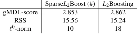
SparseL2Boost (#) L2Boosting

gMDL-score 2.853 2.862

RSS 15.56 15.24

ℓ0_{-norm 10 18}

Table 5: Boosting with componentwise linear least squares for ozone data with first

order-interactions (n=330, p=45). gMDL-score, n−1_×residual sum of squares (RSS) and

number of selected terms (ℓ0_{-norm). (#) gMDL-sel-L}

2Boost selects SparseL2Boost as the better method.

In summary, while SparseL2Boost is about as good as L2Boosting in terms of predictive accu-racy, see Table 4, it yields a sparser model fit, see Tables 4 and 5.

3.3 Binary Tumor Classification Using Gene Expressions

We consider a real data set which contains p=7129 gene expressions in 49 breast tumor samples

using the Affymetrix technology, see West et al. (2001). After thresholding to a floor of 100 and a ceiling of 16,000 expression units, we applied a base 10 log-transformation and standardized each

experiment to zero mean and unit variance. For each sample, a binary response variable Y _{∈ {}0,1_}

is available, describing the status of lymph node involvement in breast cancer. The data are available athttp://mgm.duke.edu/genome/dna micro/work/.

Although the data has the structure of a binary classification problem, the squared error loss is

quite often employed for estimation. We use L2Boosting and SparseL2Boost with componentwise

linear least squares. We classify the label 1 if ˆp(x) =Pˆ[Y+1_|X=x]>1/2 and zero otherwise. The estimate for ˆp(_·)is obtained as follows:

ˆ

pm(·) =1/2+Fˆm(·), ˆ

Fm(·)the L2- or SparseL2Boost estimate using ˜Y=Y−1/2. (20)

zero. When using L2- or SparseL2Boost on Y ∈ {0,1}directly, with an intercept term, we would obtain a shrunken boosting estimate of the intercept introducing a bias rendering ˆp(_·)to be system-atically too small. The latter approach has been used in B¨uhlmann (2006) yielding worse results for L2Boosting than what we report here for L2Boosting using (20).

Since the gMDL criterion is relatively new, its classification counterpart is not yet well devel-oped (see Hansen and Yu, 2002). Instead of the gMLD criterion in (14) and (15), we use the BIC score for the Bernoulli-likelihood in a binary classification:

BIC(m) =₋2_·log-likelihood+log(n)_·trace(Bm).

The AIC criterion would be another option: it yields similar, a bit less sparse results for our tumor classification problem.

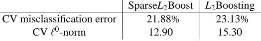
We estimate the classification performance by a cross-validation scheme where we randomly divide the 49 samples into balanced training- and test-data of sizes 2n/3 and n/3, respectively, and we repeat this 50 times. We also report on the average of selected predictor variables. The reports are given in Table 6.

SparseL2Boost L2Boosting

CV misclassification error 21.88% 23.13%

CVℓ0_{-norm 12.90 15.30}

Table 6: Boosting with componentwise linear least squares for tumor classification data (n=

46, p=7129). Misclassification error and average number of selected predictor variables

using cross-validation (with random 2/3 training and 1/3 test sets).

The predictive performance of L2- and SparseL2Boosting compares favourably with four other

methods, namely 1-nearest neighbors, diagonal linear discriminant analysis, support vector machine

with radial basis kernel (from the R-package e1071and using its default values), and a forward

selection penalized logistic regression model (using some reasonable penalty parameter and number of selected genes). For 1-nearest neighbors, diagonal linear discriminant analysis and support vector machine, we pre-select the 200 genes which have the best Wilcoxon score in a two-sample problem (estimated from the training data set only), which is recommended to improve the classification performance. Forward selection penalized logistic regression is run without pre-selection of genes. The results are given in Table 5 which is taken from B¨uhlmann (2006).

FPLR 1-NN DLDA SVM

CV misclassification error 35.25% 43.25% 36.12% 36.88%

Table 7: Cross-validated misclassification rates for lymph node breast cancer data. Forward variable selec-tion penalized logistic regression (FPLR), 1-nearest-neighbor rule (1-NN), diagonal linear discrim-inant analysis (DLDA) and a support vector machine (SVM)

When using SparseL2Boost and L2Boosting on the whole data set, we get the following results

of the 14 selected variables (genes) from L2Boosting. Analogously as in section 3.2, we give some ANOVA-type numbers of SparseL2Boosting: the error variability is n−1∑n_i=1(Yi−Yˆi)2=0.052 and

the goodness of fit equals R2=∑n

i=1(Yˆi−Y)2/∑ni=1(Yi−Y)2 =0.57, where ˆYi =Fˆ(Xi) and Y = n−1∑n_i=1Yi.

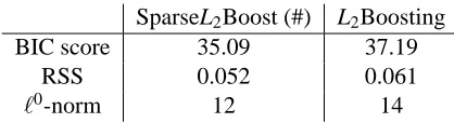
SparseL2Boost (#) L2Boosting

BIC score 35.09 37.19

RSS 0.052 0.061

ℓ0_{-norm 12 14}

Table 8: Boosting with componentwise linear least squares for tumor classification (n=49, p=

7129). BIC score, n−1_× residual sum of squares (RSS) and number of selected terms

(ℓ0_{-norm). (#) BIC-sel-L}

2Boost selects SparseL2Boost as the better method.

In summary, the predictive performance of SparseL2Boost is slightly better than of L2Boosting, see Table 6, and SparseL2Boost selects a bit fewer variables (genes) than L2Boosting, see Tables 7 and 8.

3.4 Nonparametric Function Estimation with Second-Order Interactions

Consider the Friedman #1 model Friedman (1991),

Y =10 sin(πX1X2) +20(X3−0.5)2+10X4+5X5+ε,

X_∼Unif.([0,1]p),ε_∼

N

(0,1), (21)

whereεis independent from X . The sample size is chosen as n=50 and the predictor dimension is

p_{∈ {}10,20_}which is still large relative to n for a nonparametric problem.

SparseL2Boost and L2Boosting with a pairwise thin plate spline, which selects the best pair of predictor variables yielding lowest residual sum of squares (when having the same degrees of

freedom d.f.=_{5 for every thin plate spline), yields a second-order interaction model; see also}

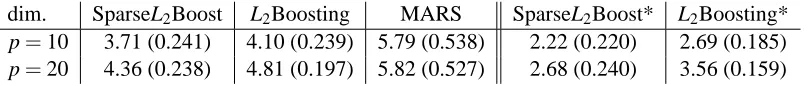
section 2.1. We demonstrate in Table 9 the effectiveness of these procedures, also in comparison

with the MARS Friedman (1991) fit constrained to second-order interaction terms. SparseL2Boost

is a bit better than L2Boosting. But the estimation of the boosting iterations by gMDL did not do as well as in section 3.1 since the oracle methods perform significantly better. The reason is that this example has a high signal to noise ratio. From (Hansen and Yu, 1999), the F in the gMDL penalty (see (14)) is related to the signal to noise ratio (SNR). Thus, when SNR is high, the log(F)is high too, leading to too small models in both SparseL2Boost and L2Boosting: that is, this large penalty

forces both SparseL2Boost and L2Boosting to stop too early in comparison to the oracle stopping

iteration which minimizes MSE. However, both boosting methods nevertheless are quite a bit better than MARS.

When increasing the noise level, using Var(ε) =16, we obtain the following MSEs for p=10:

11.70 for SparseL2Boost, 11.65 for SparseL2Boost* with the oracle stopping rule and 24.11 for

MARS. Thus, for lower signal to noise ratios, stopping the boosting iterations with the gMDL

dim. SparseL2Boost L2Boosting MARS SparseL2Boost* L2Boosting*

p=10 3.71 (0.241) 4.10 (0.239) 5.79 (0.538) 2.22 (0.220) 2.69 (0.185)

p=20 4.36 (0.238) 4.81 (0.197) 5.82 (0.527) 2.68 (0.240) 3.56 (0.159)

Table 9: Mean squared error (MSE) in model (21). All other specifications are described in the caption of Table 1, except for MARS which is constrained to second-order interaction terms.

4. Conclusions

We propose SparseL2Boost, a gradient descent algorithm on a penalized squared error loss which

yields sparser solutions than L2Boosting or ℓ1_{-regularized versions thereof. The new method is}

mainly useful for high-dimensional problems with many ineffective predictor variables (noise vari-ables). Moreover, it is computationally feasible in high dimensions, for example having linear complexity in the number of predictor variables p when using componentwise linear least squares or componentwise smoothing splines (see section 2.1).

SparseL2Boost is essentially as generic as L2Boosting and can be used in connection with non-parametric base procedures (weak learners). The idea of sparse boosting could also be transferred to boosting algorithms with other loss functions, leading to sparser variants of AdaBoost and Log-itBoost.

There is no general superiority of sparse boosting over boosting, even though we did find in four out of our five examples (two real data and two synthetic data sets) that SparseL2Boost outperforms L2Boosting in terms of sparsity and SparseL2Boost is as good or better than L2Boosting in terms of predictive performance. In the synthetic data example in section 3.1.2, chosen to be the ideal

situation for L2Boosting, SparseL2Boost loses 70% in terms of MSE, but uses only 1/3 of the

pre-dictors. Hence if one cares about sparsity, SparseL2Boost seems a better choice than L2Boosting. In our framework, the boosting approach automatically comes with a reasonable notion for statistical complexity or degrees of freedom, namely the trace of the boosting operator when it can be ex-pressed in hat matrix form. This trace complexity is well defined for many popular base procedures (weak learners) including componentwise linear least squares and decision trees, see also section 2.1. SparseL2Boost gives rise to a direct, fast computable estimate of the out-of-sample error when combined with the gMDL model selection criterion (and thus, by-passing cross-validation). This out-of-sample error estimate can also be used for choosing the stopping iteration in L2Boosting and for selecting between sparse and traditional boosting, resulting in the gMDL-sel-L2Boost algorithm.

Theoretical results in the orthogonal linear regression model as well as simulation and data

experiments are provided to demonstrate that the SparseL2Boost indeed gives sparser model fits

than L2Boosting and that gMDL-sel-L2Boost automatically chooses between the two to give a rather satisfactory performance in terms of sparsity and prediction.

5. Proofs

Proof of Theorem 2. We represent the componentwise linear least squares base procedure as a hat operator

H

_Sˆ with

H

_j =x(j)(x(j)₎T_{, where x}(j)_{= (x}(j)

1 , . . . ,x

(j)

n )T; see also section 2.1. The

L2Boosting operator in iteration m is then given by the matrix

B

_m=I₋(I₋ν

H

₁)m1_(I−ν

_H

2)m2···(I−ν

H

n)mn,

where mi equals the number of times that the ith predictor variable has been selected during the m

boosting iterations; and hence m=∑n_i=1mi. The derivation of the formula above is straightforward because of the orthogonality of the predictors x(j)and x(k)which implies the commutation

H

_j

H

_k=

H

_k

H

_j. Moreover,

B

_mcan be diagonalized

B

_m=XDmXT with XTX=XXT =I,Dm=diag(dm,1, . . . ,dm,n), dm,i=1−(1−ν)mi. Therefore, the residual sum of squares in the mth boosting iteration is:

RSSm=kY−

B

mYk2=kXTY−XT

B

mYk2=kZ−DmZk2=k(I−Dm)Zk2,

where Z=XTY.

The RSSm decreases monotonically in m. Moreover, the amount of decrease RSSm−RSSm+1

is decaying monotonously in m, because L2Boosting proceeds to decrease the RSS as much as

possible in every step (by selecting the most reducing predictor x(j)) and due to the structure of (1₋dm,i) = (1−ν)mi. Thus, every stopping of boosting with an iteration number m corresponds to a toleranceδ2such that

RSSk−RSSk+1>δ2,k=1,2, ...,m−1,

RSSm−RSSm+1≤δ2, (22)

that is, the iteration number m corresponds to a numerical tolerance where the difference RSSm−

RSSm+1is smaller thanδ2.

Since L2Boosting changes only one of the summands in RSSmin the boosting iteration m+1,

the criterion in (22) implies that for all i_{∈ {}1, . . . ,n_}

((1₋ν)2(mi−1)₋₍₁₋ν₎2mi_)Z2

i >δ2,

((1₋ν)2mi₋₍₁₋ν₎2(mi+1)_)Z2

i ≤δ2. (23)

If mi=0, only the second line in the above expression is relevant. The L2Boosting solution with

toleranceδ2is thus characterized by (23).

Let us first, for the sake of insight, replace the “_≤” in (23) by “_≈”: we will deal later in which

sense such an approximate equality holds. If mi≥1, we get

((1₋ν)2mi₋₍₁₋ν₎2(mi+1)_)Z2

i = (1−ν)2mi(1−(1−ν)2)Zi2≈δ2, and hence

(1₋ν)mi _≈ δ p

1−(1−ν)2_|Z i|

In case where mi=0, we obviously have that 1−(1−ν)mi=0. Therefore,

ˆ

β(m)

Boost,i=Zˆi=dm,i= (1−(1−ν)mi)Zi≈Zi−

δ p

1₋(1₋ν)2_|Z i|

Zi if m1≥1,

ˆ

β(m)

Boost,i=0 if mi=0.

Since mi=0 happens only if|Zi| ≤ √ δ

1−(1−ν)2, we can write the estimator as

ˆ

β(m)

Boost,i≈



 

 

Zi−λ, if Zi≥λ, 0, if_|Zi|<λ,

Zi+λ, if Zi≤ −λ.

(25)

whereλ=√ δ

1−(1−ν)2 (note that m is connected toδ, and hence toλvia the criterion in (22)). This

is the soft-threshold estimator with thresholdλ, as in (13). By choosingδ=λn

p

1₋(1₋ν)2_{, we} get the desired thresholdλn.

We will now deal with the approximation in (24). By the choice ofδtwo lines above, we would

like that

(1₋ν)mi _≈λ

n/|Zi|.

As we will see, this approximation is accurate when choosingνsmall. We only have to deal with

the case where _|Zi|>λn; if|Zi| ≤λn, we know that mi=0 and ˆβi =0 exactly, as claimed in the right hand side of (25). Denote by

Vi=V(Zi) =

λn

|Zi|∈

(0,1).

(The range(0,1)holds for the case we are considering here). According to the stopping criterion in (23), the derivation as for (24) and the choice ofδ, this says that

(1₋ν)mi_>V

i,

(1−ν)mi+1_≤V

i, (26)

and hence

∆(ν,Vi)

def

= ((1₋ν)mi_−V

i)≤((1−ν)mi−(1−ν)mi+1)

= ν

1₋ν(1−ν)

mi+1_≤ ν

1₋νVi,

by using (26). Thus,

(1₋ν)mi_=V

i+ ((1−ν)mi−Vi) =Vi(1+∆(ν,Vi)/Vi) =Vi(1+ei(ν)),

|ei(ν)|=|∆(ν,Vi)/Vi| ≤ν/(1−ν). (27)

Thus, when multiplying with(₋1)Ziand adding Zi,

ˆ

β(m)

Boost,i = (1−(1−ν)mi)Zi=Zi−ZiVi(1+ei(ν))

where max1_≤i≤n|ei(ν)| ≤ν/(1−ν)as in (27). 2

Proof of Theorem 1. The proof is based on similar ideas as for Theorem 2. The SparseL2Boost in iteration m aims to minimize

MSBm=RSSm+γntrace(Bm) =kY−X ˆβ( m)

ms₋boostk 2_+γ

ntrace(Bm).

When using the orthogonal transformation by multiplying with XT, the criterion above becomes

MSBm=kZ−βˆ_ms(m₋)_boostk2+γntrace(Bm),

where trace(Bm) =∑ni=1(1−(1−ν)mi). Moreover, we run SparseL2Boost until the stopping itera-tion m satisfies the following:

MSBk−MSBk+1>0, k=1,2, . . . ,m−1,

MSBm−MSBm+1≤0. (28)

It is straightforward to see for the orthonormal case, that such an m coincides with the definition for ˆ

m in section 2.3. Since SparseL2Boost changes only one of the summands in RSS and the trace of

B

_m, the criterion above implies that for all i=1, . . . ,n, using the definition of MSB,

(1₋ν)2(mi−1)_Z2

i(1−(1−ν)2)−γnν(1−ν)mi−1>0,

(1₋ν)2mi_Z2

i(1−(1−ν)2)−γnν(1−ν)mi≤0. (29) Note that if_|Zi|2≤γnν/(1−(1−ν)2), then mi=0. This also implies uniqueness of the iteration m such that (28) holds or of the misuch that (29) holds.

Similarly to the proof of Theorem 2, we look at this expression first in terms of an approximate equality to zero, that is_≈0. We then immediately find that

(1₋ν)mi _≈ γnν

(1−(1−ν)2_)|Z i|2

.

Hence,

ˆ

β(m)

ms−boost,i = (X T

_B

mY)i= (XTXDmXTY)i= (DmZ)i= (1−(1−ν)mi)Zi

≈ Zi−

γnνZi

(1₋(1₋ν)2_)|Z i|2

=Zi−sign(Zi)

γn

2₋ν

1

|Zi|

.

The right-hand side is the nonnegative garrote estimator as in (12) with thresholdγn/(2−ν).

Dealing with the approximation “_≈” can be done similarly as in the proof of Theorem 2. We

define here

Vi=V(Zi) =

γnν

(1₋(1₋ν)2_)|Z i|2

.

We then define∆(ν,Vi)and ei(ν) as in the proof of Theorem 2, and we complete the proof as for

Theorem 2. 2

B. Yu would like to acknowledge gratefully the partial supports from NSF grants FD01-12731 and CCR-0106656 and ARO grants DAAD19-01-1-0643 and W911NF-05-1-0104, and the Miller Re-search Professorship in Spring 2004 from the Miller Institute at University of California at Berkeley. Both authors thank David Mease, Leo Breiman, two anonymous referees and the action editors for their helpful comments and discussions on the paper.

References

H. Akaike. Statistical predictor identification. Ann. Inst. Statist. Math., 22:203, 1970.

L. Breiman. Better subset regression using the nonnegative garrote. Technometrics, 37:373–384, 1995.

L. Breiman. Bagging predictors. Machine Learning, 24:123–140, 1996.

L. Breiman. Arcing classifiers (with discussion). Ann. Statist., 26:801–849, 1998.

L. Breiman. Prediction games & arcing algorithms. Neural Computation, 11:1493–1517, 1999.

P. B¨uhlmann. Boosting for high-dimensional linear models. To appear in Ann. Statist., 34, 2006.

P. B¨uhlmann and B. Yu. Boosting with the l2loss: regression and classification. J. Amer. Statist. Assoc., 98:324–339, 2003.

B. Efron, T. Hastie, I. Johnstone, and R. Tibshirani. Least angle regression (with discussion). Ann. Statist., 32:407–451, 2004.

Y. Freund and R. E. Schapire. Experiments with a new boosting algorithm. In Machine Learning: Proc. Thirteenth Intern. Conf., pages 148–156. Morgan Kauffman, 1996.

J. H. Friedman. Greedy function approximation: a gradient boosting machine. Ann.Statist., 29: 1189–1232, 2001.

J. H. Friedman. Multivariate adaptive regression splines (with discussion). Ann.Statist., 19:1–141, 1991.

J. H. Friedman, T. Hastie, and R. Tibshirani. Additive logistic regression: a statistical view of boosting (with discussion). Ann. Statist., 28:337–407, 2000.

P. J. Green and B. W. Silverman. Nonparametric Regression and Generalized Linear Models: A Roughness Penalty Approach. Chapman and Hall, 1994.

M. Hansen and B. Yu. Model selection and minimum description length principle. J. Amer. Statist. Assoc., 96:746–774, 2001.

M. Hansen and B. Yu. Minimum Description Length Model Selection Criteria for Generalized Linear Models. IMS Lecture Notes – Monograph Series, Vol. 40, 2002.

G. Lugosi and N. Vayatis. On the bayes-risk consistency of regularized boosting methods (with discussion). Ann. Statist., 32:30–55 (disc. pp. 85–134), 2004.

S. Mallat and Z. Zhang. Matching pursuits with time-frequency dictionaries. IEEE Trans. Signal Proc., 41:3397–3415, 1993.

N. Meinshausen. Lasso with relaxation. Technical report, 2005.

G. R¨atsch, T. Onoda, and K.-R. M¨uller. Soft margins for adaboost. Machine Learning, 42:287–320., 2001.

G. R¨atsch, A. Demiriz, and K. Bennett. Sparse regression ensembles in infinite and finite hypothesis spaces. Machine Learning, 48:193–221, 2002.

T. Speed and B. Yu. Model selection and prediction: normal regression. Ann. Inst. Statist. Math., 45:35–54, 1993.

R. Tibshirani. Regression shrinkage and selection via the lasso. J. Roy. Statist. Soc., Ser. B, 58: 267–288, 1996.

J. W. Tukey. Exploratory data analysis. Addison-Wesley, 1977.