Multitask Sparsity via Maximum Entropy Discrimination

Multitask Sparsity via Maximum Entropy Discrimination

Tony Jebara [email protected]

Department of Computer Science Columbia University

New York, NY 10027, USA

Editor: Francis Bach

Abstract

A multitask learning framework is developed for discriminative classification and regression where multiple large-margin linear classifiers are estimated for different prediction problems. These clas-sifiers operate in a common input space but are coupled as they recover an unknown shared rep-resentation. A maximum entropy discrimination (MED) framework is used to derive the multitask algorithm which involves only convex optimization problems that are straightforward to implement. Three multitask scenarios are described. The first multitask method produces multiple support vec-tor machines that learn a shared sparse feature selection over the input space. The second multitask method produces multiple support vector machines that learn a shared conic kernel combination. The third multitask method produces a pooled classifier as well as adaptively specialized individual classifiers. Furthermore, extensions to regression, graphical model structure estimation and other sparse methods are discussed. The maximum entropy optimization problems are implemented via a sequential quadratic programming method which leverages recent progress in fast SVM solvers. Fast monotonic convergence bounds are provided by bounding the MED sparsifying cost function with a quadratic function and ensuring only a constant factor runtime increase above standard inde-pendent SVM solvers. Results are shown on multitask data sets and favor multitask learning over single-task or tabula rasa methods.

Keywords: meta-learning, support vector machines, feature selection, kernel selection, maximum

entropy, large margin, Bayesian methods, variational bounds, classification, regression, Lasso, graphical model structure estimation, quadratic programming, convex programming

1. Introduction

In applied domains ranging from biology to vision, inter-related data is collected by researchers for varying scientific purposes. While there are some concerted efforts to ensure that data sets are collected and labeled in consistent ways, it is often the case that many heterogeneous data sets over a given input domain are collected and labeled for different tasks. Most machine learning approaches take a single-task perspective where one large homogeneous repository of uniformly collected iid (independent and identically distributed) samples is given and labeled consistently. A more realistic,

multitask learning approach is to combine data from multiple smaller sources and synergistically

leverage heterogeneous labeling or annotation efforts.

dependen-cies and redundandependen-cies when compared to another data set. Single-task learning from each data set in isolation (in a tabula rasa inductive manner) provides only a narrow view of the phenomenon at hand. Meanwhile, multitask learning (or inductive transfer) uses the collection of data sets simul-taneously to exploit the related nature of the problems. For example, a multitask learning approach may involve algorithms that discover shared representations that are useful across several data sets and tasks. For instance, consider a group of doctors each interested in predicting the presence or absence of a particular disease from a set of medical tests that can be performed on a patient. Since medical tests may be invasive and expensive, the doctors may wish to find a small subset of medical tests (the shared representation) that can be performed on a patient once and for all such that each disease of interest can be accurately predicted.

This article explores maximum entropy discrimination approaches to multitask problems and is organized as follows. Section 2 reviews previous work in multitask learning, support vector machine feature selection and support vector machine kernel selection. Section 3 sets up the general multi-task problem as learning from data that has been sampled from a set of generative models that are dependent given data observations yet become independent given a shared representation. Section 4 migrates the standard Bayesian treatment of the problem into a large-margin discriminative setting using maximum entropy. The log-linear model, the main classifier of interest in this article, is expli-cated in Section 5. Section 6 explicates the case where the shared representation is a binary feature selection that removes certain input space features in a consistent manner for all linear classification tasks. Section 7 extends the shared representation such that it explores any conic kernel combination with multiple linear classifiers. Section 8 extends the framework to adaptive data pooling problems. Section 9 illustrates the corresponding derivations in a multitask (scalar) regression setting. Sec-tion 10 briefly describes the sequential quadratic programming method which is to be applied to the convex programs derived in the various preceding sections. Experimental results are provided in Section 11. An extension that permits the approach to perform sparse graph structure estimation is described in Section 12 and Section 13 then concludes with a brief summary. The Appendix pro-vides the derivation of a bound which converts all the necessary optimization steps into quadratic programming with a proof of fast convergence for the resulting sequential quadratic programming procedure. The Appendix also discusses connections to other sparse regression methods.

2. Previous Work

Since this article involves the combination of the three research areas, we review previous work in multitask learning, support vector machine (SVM) feature selection and SVM kernel selection.

learning by assuming dependencies between the various models and tasks (Heskes, 1998, 2004). For instance, tasks can be clustered via a hierarchical mixture of Gaussians which couples their parameters. In addition, some theoretical arguments for the benefits of multitask learning have been made (Baxter, 2000) showing that the average error of M tasks can potentially decrease inversely with M. More recently, improved generalization guarantees for each individual task were provided if the classifiers are related and share a common structure (Ben-David and Schuller, 2003).

Concurrently, kernel methods (Sch¨olkopf and Smola, 2001) and large-margin support vector machines are highly successful in single-task settings and are good candidates for multitask exten-sions. While multiclass variants of binary classifiers have been extensively explored (Crammer and Singer, 2001), multitask classification differs in that it often involves distinct sets of input data for each task. Furthermore, the concept of shared representation has been less practical to implement for kernel methods and support vector machines. For example, constraining the representation by performing SVM feature selection in a single-task setting may require extensions beyond standard quadratic programming (Jebara and Jaakkola, 2000; Weston et al., 2000). Similarly, constraining a representation to perform SVM kernel selection is also more involved in a single-task setting and requires second-order cone programming or semidefinite programming (Cristianini et al., 2001; Lanckriet et al., 2002).

This article focuses on multitask extensions of both feature selection and kernel selection with support vector machines. The derivations here will closely follow previous work which migrated maximum entropy to single-task SVMs (Jaakkola et al., 1999), to sparse SVMs (Jebara and Jaakkola,

2000) and to multitask SVMs (Jebara, 2003, 2004).1 This maximum entropy framework led to one

of the first convex large margin multitask classification approaches (Jebara, 2004). Convexity was subsequently explored in other multitask frameworks (Argyriou et al., 2008). The present arti-cle extends the derivations in the maximum entropy discrimination multitask approach, provides a straightforward iterative quadratic programming implementation and uses tighter bounds for im-proved runtime efficiency. Other related multitask SVM approaches have also been promising in-cluding novel kernel construction techniques to couple tasks (Evgeniou et al., 2005). These permit standard SVM learning algorithms to perform multitask learning while the multitask issues are han-dled primarily by the kernel itself. Even more recently, online algorithms have been proposed (Dekel et al., 2006) for multitask learning with margin-based predictors and provide interesting worst-case guarantees. Extensions to handle unlabeled data in multitask settings have also been promising (Ando and Zhang, 2005) and enjoyed theoretical generalization guarantees. An alternative per-spective to multitask feature and kernel selection can be explored by performing joint covariate or subspace selection for multiple classification problems (Obozinski et al., 2010). Furthermore, fea-ture selection and kernel selection can be seen as sparsity inducing methods. While a survey of sparsity is out of the scope of this article, one of the most popular implementations of sparsity or selection in regression settings is theℓ1regularized Lasso method and its variants (Tibshirani, 1996; Tropp, 2006). Therein, sparsity is usually explored in a single-task setting and is used to remove unnecessary features in a regression problem (although sparsity is equally relevant in classification problems Jebara and Jaakkola, 2000). The multitask extension to such sparse estimation techniques is known as the Group Lasso and allows sparsity to be explored over predefined subsets of variables (Turlach et al., 2005; Yuan and Lin, 2006). Consistency arguments and connections between the Group Lasso and multiple kernel learning were also provided (Bach et al., 2004; Bach, 2008).

sity and its connection to maximum entropy discrimination and so-called Laplace Markov networks was also recently explored (Zhu et al., 2008). This article provides another contact point between sparsity, large margins, multitask learning and kernel selection. The next sections formulate the general probabilistic setup for such multitask problems and convert traditional Bayesian solutions into a discriminative large-margin setting using the maximum entropy framework (Jaakkola et al., 1999).

3. Multitask Learning

The general multitask learning setup is as follows. We are given a collection of data sets

D

=

{

D

1, . . . ,

D

M}covering m=1. . .M tasks. Each task has its training set

D

m of t=1. . .Tm

input-output pairs(xm,t,ym,t)that are independent and identically distributed (iid) samples from an

un-known probability density function

P

m defined jointly over both inputs and outputs. The data for

task m is therefore

D

m={(xm,1,ym,1), . . . ,(xm,Tm,ym,Tm)}. The inputs may be in a Euclidean vector

space xm,t∈RDor, more generally, xm,t∈

X

are objects that could be mapped to a Hilbert space via

a kernel. In a regression setting we assume the outputs are scalars ym,t ∈Rwhile in a classification

setting we would assume binary2outputs ym,t∈ {±1}.

There are many ways to tie together multiple inter-related tasks synergistically. In this section and in Section 4, it will be helpful to take a Bayesian perspective to the multitask problem although this perspective is not strictly necessary in subsequent sections. From a Bayesian point of view, several model parameters will be estimated and assumed to be random variables governed by a

dis-tribution and priors. Assume that there are task-specific model parametersΘm associated to each

task or data set

D

mfor m=1. . .M. The single-task or tabula rasa learning approach assumes that

the models are independent given their respective data sets and, therefore, can be recovered inde-pendently. Such an assumption may be too simple in practice. The more general multitask learning assumption is that there exist dependencies between the tasks. In other words, the likelihood of the models given the data does not factorize,

p(Θ1, . . . ,ΘM|

D

) 6=

M

∏

m=1

p(Θm|

D

m).

One specific way of coupling the various parametersΘ1, . . . ,ΘM is to instead assume that there is

another parameter s that is shared across tasks. For example, s could be a set of binary switches that eliminate all but a few features in the input space. The models then become independent only if the

shared parameter3or representation is observed as follows:

p(Θ1, . . . ,ΘM|s,

D

) =

M

∏

m=1

p(Θm|s,

D

m).

Note that, given data, the models are conditionally independent given the representation yet are dependent otherwise. This lack of factorization is on the posterior when data is observed, not on

2. In this article, only the binary classification case will be considered, however, the techniques herein extend easily to multiclass settings where ym,t∈ {1, . . . ,Y}with Y∈Zand Y ≥3. Alternatively, it is straightforward to use binary

classification methods on multiclass problems by using Y one-versus-all binary classifiers, by using Y(Y−1)/2 one-versus-one binary classifiers, or by using error-correcting codes (Dietterich and Bakiri, 1995).

the prior. We may still make the assumption that p(Θ) factorizes a priori. However, observing data with a latent shared parameter s induces dependencies across the multiple tasks. In terms of a directed acyclic graph where the joint probability density function factorizes as a product of nodes given their parents, the following dependency structure emerges in the (simplest) case of multitask

learning with two models: Θ1→

D

1←s→

D

2←Θ2. Therefore, observing the data

D

1 and

D

2

couples the two models unless the shared representation s is also observed.

Thus, a natural way of exploring dependencies between tasks is to assume a shared represen-tation variable s is implicated in the learning problem. We then have a total set of parameters

Θ={Θ1, . . . ,ΘM,s}to jointly estimate from all the data sets. We explore the following scenarios:

• Feature Selection: Consider M individual modelsΘm={θm,bm}which are linear classifiers

whereθm∈RDand bm∈R. The shared representation s∈BD is a binary feature selection

vector that either keeps (s(d) =1) or eliminates (s(d) =0) each input vector dimension.

• Kernel Selection: Consider M individual models Θm ={θm,1, . . . ,θm,D,bm} where each

modelΘmconsists of D linear classifiers in D different Hilbert spaces and one scalar bm∈R.

The shared configuration s∈BD_{is a binary feature selection vector that either keeps (when}

s(d) =1) or eliminates (when s(d) =0) the candidate Hilbert space from the classifiers.

• Adaptive Pooling: Consider M+1 different linear classification models where M tasks have to choose between using their own specialized classifierθ1, . . . ,θM or a communal classifier

θby estimating s∈BM, a binary selection vector.

• Graphical Model Structure: Consider estimating from sample data a graphical model struc-ture over D random variables by finding D classifiers that predict each variable from all others.

The following sections detail these multitask learning scenarios and show how we can learn discriminative classifiers (that predict outputs accurately and with large margin) from multiple tasks. To tackle this problem, we will apply the maximum entropy discrimination framework (Jaakkola et al., 1999) since it produces convex optimization problems where global optima can be reliably recovered. Furthermore, the framework produces large margin discrimination and thus inherits the performance benefits of support vector machines.

4. Bayes and Maximum Entropy

The standard Bayesian approach to inference begins with a prior p(Θ)over a model classΘ(which

can be possibly uncountable or continuous). The prior is then refined given the data to obtain a posterior p(Θ|

D

)via Bayes’ rule p(Θ|

D

)∝p(

D

|Θ)p(Θ). Subsequently, the posterior is used to make predictions for new observations. The Bayesian prediction of a label for a new query input x for task m is as follows:

ˆ

y=arg max

y Z

p(y|x,Θm)p(Θ|

D

)dΘ. (1)

In the above, a prediction ˆy is obtained from the predictive distribution p(y|x,Θm) by integrating over all modelsΘwhile weighing each predictive distribution by the posterior p(Θ|

D

). This poste-rior, according the Bayes rule, is simply the product of the prior and the likelihood as follows:

p(Θ|

D

) = 1 Zp(Θ)

M

∏

m=1

Tm

∏

t=1

Previous approaches (Heskes, 2004) followed such a Bayesian treatment for multitask learning and obtained promising results. In this article, however, we will modify the standard Bayesian posterior to learn a more discriminative solution. Instead of using Bayes’ rule to infer the posterior, we

con-sider a posterior which produces predictions ˆy with large margin as in the support vector machine

(SVM) framework (Cortes and Vapnik, 1995). In other words, we will construct a discriminative posterior density which yields both accurate classification and large margins when used in Equa-tion 1. Accurate classificaEqua-tion on the observed data is obtained by forcing the marginal likelihood of the correct label ym,t to be larger than that of incorrect labels for each observation t=1, . . . ,Tmin

all m=1, . . . ,M data sets:

Z

p(ym,t|xm,t,Θm)p(Θ|

D

)dΘ−max y6=ym,t Z

p(y|xm,t,Θm)p(Θ|

D

)dΘ ≥ 0.

This ensures that the posterior gives good predictions on average since the correct label ym,t has a

higher probability than the wrong label (Crammer and Singer, 2001; Taskar et al., 2004). The above constraints require that the likelihood of the correct label remain larger than the likelihood of the

incorrect label on average under the posterior over Θ. We consider one additional simplification

for computational considerations. Instead of comparing likelihoods, we will require that the

log-likelihood of the correct label is larger than the log-log-likelihood of the incorrect label on average

under the posterior overΘ. Furthermore, to achieve large margin, we will force the posterior to

not only make correct predictions but to also produce a score for the correct label that is at least a

constantγabove the value obtained by incorrect labels:

Z

log p(ym,t|xm,t,Θm)p(Θ|

D

)dΘ−max y6=ym,t Z

log p(y|xm,t,Θm)p(Θ|

D

)dΘ ≥ γ.

In many parts of this article, without loss of generality, we will assume thatγ=1. These

correct-classification constraints are applied to all training data t=1, . . . ,Tmfor all tasks m=1. . .M. Such

classification or discrimination constraints were first introduced in the so-called maximum entropy discrimination (MED) framework (Jaakkola et al., 1999) and give rise to posterior distributions that mimic support vector machines and large-margin learning. The MED framework also conveniently leads to analytic expressions and closed-form solutions for all the necessary integrals. Instead of using Bayes rule to obtain the posterior, MED finds a posterior that is as close as possible to the prior in terms of Kullback-Leibler Divergence. In other words, it minimizes the relative entropy to the prior KL(p(Θ|

D

)kp(Θ))but still also satisfies the above classification constraints. This produces the following primal optimization problem:

O

primal

(

minP(Θ|D)KL(p(Θ|

D

)kp(Θ))

s.t. Rlog _p(ym

,t|xm,t,Θm) p(y|xm,t,Θm)

p(Θ|

D

)dΘ≥γ ∀y6=ym,t,m,t.

The solution is straightforward and gives the following posterior:

p(Θ|

D

) = 1 Z(λ)p(Θ)

M

∏

m=1

Tm

∏

t=1y6=

∏

ym,t

p(ym,t|xm,t,Θm) p(y|xm,t,Θm)

λm,t

exp(−γλm,t). (2)

Here,λis a collection (or a vector) of non-negative Lagrange multipliers{λm,t}for m=1, . . . ,M

posterior is Z(λ). Maximum entropy solves for the Lagrange multipliers by maximizing J(λ) = −log Z(λ). This is simply the dual optimization

O

dual

maxλ_≥0−log

R

p(Θ)∏M_m=1∏Tm_t=1∏y_6=ym,tp(ym,t|xm,t,Θm) p(y|xm,t,Θm)

λm,t

exp(−γλm,t)dΘ.

If all λm,t are set to 1, the posterior resembles the standard Bayesian estimate. However, MED

estimates different weightsλm,t for each datum (or classification constraint) in the posterior. This

ensures that the classification constraints are achieved. Instead of treating all points equally, the MED solution explores weights on each datum to adjust the Bayesian solution such that it obtains better classification on the training data. The expected log-likelihood of the data under the MED posterior satisfies the classification constraints while staying close to the prior. Furthermore, MED uses the expected log-likelihood of a new query point to make predictions as follows:

ˆ

y = arg max

y Ep(Θ|D)[log p(y|x,Θm)] = arg maxy Z

log p(y|x,Θm)p(Θ|

D

)dΘ.

This simple reformulation of the standard Bayesian posterior will give rise to large margin learning as explicated in the next section.

5. From Log-Linear Models to Support Vector Machines

We next make more specific assumptions on the form of the predictive distribution p(y|x,Θm).

Assume that the predictive distribution is log-linear as follows:

p(y|x,Θm) ∝ exp y

2hx,θmi+bm)

.

This permits us to rewrite the above posterior p(Θ|

D

)more specifically as:

p(Θ|

D

) = 1 Z(λ)p(Θ)

M

∏

m=1

Tm

∏

t=1

exp(ym,t(hxm,t,θmi+bm))λm,texp(−γλm,t).

We integrate the above overΘ={Θ1, . . . ,ΘM,s}to obtain the partition function Z(λ). The objective function we need to maximize is the negative logarithm of the partition function:

J(λ) = −log

Z

p(Θ)exp

M

∑

m=1

Tm

∑

t=1

λm,tym,t(hxm,t,θmi+bm)−γλm,t

!

dΘ.

We will next assume that the prior over models factorizes as follows:

p(Θ) = p(s) M

∏

m=1

p(Θm) = p(s) M

∏

m=1

N

(θm|0,I)

N

(bm|0,σ2).

couple the models in the posterior. However, in this first example we will not obtain any coupling per se. This is clear once we evaluate the integrals to obtain the objective function:

J(λ) = − M

∑

m=1

log

Z

exp(hθm,

Tm

∑

t=1

λm,tym,txm,ti)

N

(θm|0,I)dθm

− M

∑

m=1

log

Z

exp(bm Tm

∑

t=1

λm,tym,t)

N

(bm|0,σ2)dbm+ M

∑

m=1

Tm

∑

t=1

γλm,t.

Simple algebra and completion of squares4yields the objective function J(λ)which is maximized

as follows

max

λ_≥0 M

∑

m=1





Tm

∑

t=1

γλm,t−

1 2

Tm

∑

t,τ=1

λm,tλm,τym,tym,τhxm,t,xm,τi −

σ2 2

Tm

∑

t=1

λm,tym,t

!2 .

The above dual optimization problem is simply a quadratic program and is straightforward to solve.

If we further assume thatσ2→∞, which corresponds to using a non-informative prior on the bias

scalar terms bm, the objective function above gives the constraints∑tλm,tym,t=0 for all m=1. . .M.

We then get an objective function that is exactly the sum of the dual objective functions of M

independent support vector machines (ifγ=1). Thus, our dual optimization is:

max

λ_≥0 M

∑

m=1

Tm

∑

t=1

γλm,t−

1 2

Tm

∑

t,τ=1

λm,tλm,τym,tym,τk(xm,t,xm,τ) !

s.t.

Tm

∑

t=1

ym,tλm,t =0∀m.

Here, we have also replaced all inner products of two inputs x and ¯x of the formhx,¯xiwith Mercer kernel evaluations k(x,¯x). This allows us to readily accommodate nonlinear classification. Finally,

the prediction rule for a query input x given the current setting of theλvalues for the m’th model

involves integrating over the posterior which produces the following prediction:

ˆ

y = arg max

y Ep(Θ|D)[log p(y|x,Θm)] = sign Tm

∑

t=1

λm,tym,tk(x,xm,t) +ˆbm

! ,

where the ˆbmscalars are given by the Karush Kuhn Tucker (KKT) conditions. Whenever a constraint

or Lagrangian is active, the corresponding Lagrange multiplier must be strictly positiveλm,t>0 and

we expect the inequalities in the primal problem to hold exactly. Therefore, we can obtain each ˆbm

by solving

ym,t = Tm

∑

τ=1

λm,τym,τk(xm,t,xm,τ) +ˆbm

for any datum t which has a corresponding Lagrange multiplier (once the dual program halts) that satisfiesλm,t>0.

Clearly, because of additivity, updatingλm,1, . . . ,λm,Tm can be done independently ofλn,1, . . . ,

λn,Tn for any n6=m. In other words, we have tabula rasa independent learning of M independent

SVMs on all the tasks. Even the scalar biases ˆbmare obtained independently via the KKT conditions.

Therefore, to obtain multitask learning, we will need some shared representation s to couple the learning problems and give rise to a non-factorized posterior over models.

5.1 Non-Separable Case

For thoroughness, this section details the case where the classification problems are not separable; in other words, not all inequalities in the maximum entropy formulation can be achieved. In this

case, we introduce non-negative slack variablesξ={ξm,t}on each constraint with a cost of C per

unit of slack leading to the following primal optimization:

O

primal

(

min_P(Θ|D),ξKL(p(Θ|

D

)kp(Θ)) +C∑M_m=1∑Tm_t=1∑y_6=ym,tξm,t,y

s.t. Rlogp(ym,t|xm,t,Θm) p(y|xm,t,Θm)

p(Θ|

D

)dΘ≥γ−ξm,t andξm,t,y≥0 ∀y6=ym,t,m,t.

The above produces the same type of solution as Equation 2 but has a slightly different dual opti-mization:

O

dual

(

maxλ ∑M_m=1

∑Tm

t=1γλm,t−1₂∑Tmt,τ=1λm,tλm,τym,tym,τk(xm,t,xm,τ)

s.t.0≤λm,t≤C ∀m,t and ∑Tmt=1ym,tλm,t =0 ∀m

which merely bounds the Lagrange multipliers from above by C. Once again, MED mimics support vector machines (Cortes and Vapnik, 1995) in the non-separable case.

6. Feature Selection

We next explore feature selection and require x∈RDwhere D∈Z. To couple the tasks, modify the

predictive distribution for the label given the model such that it also depends on a shared variable s as follows:

p(y|x,Θm,s) ∝ exp y 2

D

∑

d=1

s(d)x(d)θm(d) +bm

!! ,

where s is a binary D-dimensional vector and the argument of a vector s(d)refers to its d’th entry. Thus, the shared representation consists of binary switches that delete or censor various entries of the x vector. If s(d) =0, then the x(d) entry is effectively set to zero. Meanwhile, if s(d) =1,

the x(d)entry remains intact. In other words, the binary vector s performs a feature selection. In

addition, assume the prior for p(s)is a product of Bernoulli distributions for each element of s,

p(s) = D

∏

d=1

ρs(d)_(1−ρ)1−s(d)_,

whereρis the a priori probability of keeping the features on. For example, settingρ=1 suggests

that all features should be on and no feature selection is to be performed. Alternatively, we can

reparametrize the prior asα=1−_ρρwhere increasingαcorresponds to sparser feature selection. A

value ofα=0 indicates no feature selection is being performed (no sparsity). Meanwhile a value of

α→∞encourages the models to discard almost all features. If we perform feature selection and use

a predictive distribution with shared s, the m=1, . . . ,M tasks will become coupled and the posterior

over models no longer factorizes. The MED solution is then

p(Θ|

D

) = 1 Z(λ)p(Θ)

M

∏

m=1

Tm

∏

t=1

exp λm,tym,t D

∑

d=1

s(d)xm,t(d)θm(d) +bm

!

−γλm,t

We compute the corresponding partition function by integrating over all modelsΘ1, . . . ,Θmas well as summing over all binary settings of s which yields

Z(λ) = Z

p(Θ)exp

M

∑

m=1

Tm

∑

t=1

λm,tym,t D

∑

d=1

s(d)xm,t(d)θm(d) +bm

!

−γλm,t

!

dΘ

= exp

∑

m σ2

2

∑

t

λm,tym,t

2

−

∑

t γλm,t

!

∏

d

1−ρ+ρe12∑m(∑tλm,tym,txm,t(d))2

.

Takingσ2→∞gives a new objective function J(λ) =−log(Z(λ))which is no longer a quadratic program yet is still a convex program as follows:

 



maxλ ∑M_m=1∑Tm_t=1γλm_,t−∑D_d=1log

α+e12∑

M

m=1(∑Tmt=1λm,tym,txm,t(d))

2

+D log(α+1)

s.t.0≤λm,t≤C ∀m,t and ∑_tT₌m₁ym,tλm,t=0 ∀m.

Note the property that J(0) =0. Clearly, the objective function is no longer additive across m=

1. . .M which means that learning is coupled across tasks. This is due to the non-linearity in the

function f(x) =log(α+exp(−x))which involves a summation over m=1. . .M. We will refer to

this function as the log-sigmoid function. If we setα=0, the log-sigmoid becomes linear and we get

back the independent optimization problems in Section 5. Therein, the tasks decouple completely (i.e., the objective function becomes additive over tasks m=1. . .M). However, larger settings ofα

encourage some coupling between the SVMs (or large margin log-linear models) as they search for a joint feature selection.

Note the presence of logarithmic terms which prevent the direct application of quadratic pro-gramming to J(λ). Fortunately, the log-sigmoid function f(x) =log(α+exp(−x))is known to be a convex function (more precisely, our objective involves a negated sum of such functions which is concave overall). Recently, new computational tools have been proposed for solving convex pro-grams that involve such terms (Koh et al., 2007). In our implementation, we instead apply a bound on the log-sigmoid to reformulate the optimization as a sequential quadratic program. Optimization

details are deferred to Section 10 but it will be assumed that a (nearly) optimalλsolution can be

recovered.

Given the recoveredλsetting, the prediction rule is straightforward to derive as follows:

ˆ

y = arg max

y Ep(Θ|D)[log p(y|x,Θm,s)] = sign D

∑

d=1

Tm

∑

t=1

λm,tym,tˆs(d)x(d)xm,t(d) +ˆbm

! .

The ˆs(d)above are expected values of s(d)under the posterior and are given by:

ˆs(d) = 1

1+αexp

−1₂∑M_m=1∑Tm_t=1λm,tym,txm,t(d)

2.

In fact, ˆs(d) are scalars in[1/(1+α),1]which give a soft feature selection as values close to the

bottom of the range are candidates for removal after thresholding. The values of ˆs(d)

multiplica-tively scale the input domain features and are close to 1/(1+α)for features that are not useful for

prediction in the multiple tasks. Once again, the ˆbmscalars are given by the KKT conditions which

require that the value inside the sign()function evaluation above exactly equals ym,t for the query

7. Kernel Selection

Feature selection and sparsity are not the only types of shared representation s one may consider. One crucial design issue of nonlinear SVMs is the choice of a kernel function. Also, kernels permit SVMs to handle non-vectorial inputs so we relax the assumption that the x inputs are Euclidean vectors and only require that they are objects from some sample space xm,t∈

X

for all m=1, . . . ,M

and t=1, . . . ,Tm. Typically, in kernel learning (Lanckriet et al., 2002), we are given a set of d=

1, . . . ,D base Mercer kernels k1, . . . ,kD where each kernel function kd:

X

×

X

→R accepts two

inputs and produces a scalar. We wish to learn a conic combination of the kernels or a sparse selection using the non-negative scalar weights w1, . . . ,wDas follows

K(x,¯x) = D

∑

d=1

wdkd(x,¯x).

Some base kernels may get a small weight and are thus not selected and others will be averaged with varying weights wd to produce a potentially better final kernel K. Each base kernel kd(x,¯x)

can be seen to correspond to a mappingφdwhich is applied to both inputs x and ¯x. The functionφd

maps an input x∈

X

to some Hilbert space we denoteΦd. The kernel is then the inner-product of

φd(x)andφd(¯x)as follows:

kd(x,¯x) = hφd(x),φd(¯x)i.

Kernel selection is equivalent to selecting some mappings and attenuating others. We thus need a shared representation vector s which is again binary and again D-dimensional to select which

kernels will be used. However, now, we have a set of M×D linear models θm,d ∈Φ∗_d for each

Hilbert space. Aθm,dvector is available for each task m=1, . . . ,M and each mapping d=1, . . . ,D.

In other words, task m has the following modeling resources on its own:Θm={θm,1, . . . ,θm,D,bm}.

The prior for the modeling resources for the m’th task is then chosen to be a product of independent white Gaussians on these D vector parameters. This leads to the following general prior for all model parameters:

p(Θ) = D

∏

d=1

ρs(d)_(1−ρ)1−s(d)

∏

M m=1

N

(θm,d|0,I)

N

(bm|0,σ2).

Once again, all tasks share and have to agree on the binary selector vector s which inherits the Bernoulli prior used in the previous section. Therefore, we have the following total set of parameters

Θ={Θ1, . . . ,ΘM,s}.

The predictive distribution for multitask kernel selection is then given by the following log-linear model (for the m’th task):

p(y|x,Θm,s) ∝ exp y 2

D

∑

d=1

s(d)hθm,d,φd(x)i+bm

!! .

We once again recover the MED posterior using Equation 2. The normalizer for the posterior Z(λ)is

then found by integrating over the parametersΘ. This multitask kernel selection objective function

J(λ)is the following convex program:

  

 

maxλ ∑M_m=1∑_tTm₌₁γλm_,t+D log(α+1)

−∑D

d=1log

α+e12∑Mm=1∑Tmt=1∑Tmτ=1λm,tλm,τym,tym,τkd(xm,t,xm,τ)

Similarly, given theλsetting, we obtain the following prediction rule:

ˆ

y = sign

D

∑

d=1

Tm

∑

t=1

λm,tym,tˆs(d)kd(x,xm,t) +ˆbm

!

where ˆs(d)are scalars that weight each kernel and are usually close to 1/(1+α)for kernels that are not beneficial for our multiple classification tasks. The weights for each kernel are recovered as:

ˆs(d) = 1

1+αexp

−1 2∑

M

m=1∑

Tm

t=1∑

Tm

τ=1λm,tλm,τym,tym,τkd(xm,t,xm,τ) .

The scalar biases ˆbmare once again recovered from the KKT conditions. From the prediction rule,

it is clear that kernel learning is effectively creating a new kernel from the base kernels as follows:

K(x,¯x) = D

∑

d=1

ˆs(d)kd(x,¯x).

When α =0, there is no coupling of tasks or sparse selection of kernels. The solution simply

corresponds to setting ˆs(d) =1 and forces the final kernel K to equal a simple sum of all base

kernels for d =1, . . . ,D. In general, however, a more appropriate final kernel could potentially

be recovered if α>0. Given such an aggregate kernel K(x,¯x), we can now write an SVM-like

prediction rule for the m’th task:

ˆ

y = sign

Tm

∑

t=1

λm,tym,tK(x,xm,t) +ˆbm

! .

Another interesting fact is that feature selection is just an instance of kernel selection. If we choose the d=1, . . . ,D kernels as follows

kd(x,¯x) = x(d)¯x(d).

we are effectively replacing kernel evaluations in this section with the scalar product of the d’th dimension of the input that was needed for feature selection. Thus, the kernel selection problem in this section clearly subsumes the feature selection problem derived in Section 6.

7.1 Independent Kernel Selection

It is possible to break the above multitask framework by allowing each task to select a combination

of kernels independently. This means that we introduce a separate sm vector for each task m=

1, . . . ,M instead of having a shared representation s. The derivation is straightforward and produces

the following convex program:

  

 

maxλ ∑M_m=1∑Tm_t=1γλm_,t+MD log(α+1)

−∑M

m=1∑Dd=1log

α+e12∑tTm=1∑Tmτ=1λm,tλm,τym,tym,τkd(xm,t,xm,τ)

s.t.0≤λm,t≤C ∀m,t and ∑tTm=1ym,tλm,t=0 ∀m

which is once again additive in m=1, . . . ,M indicating that the Lagrange multipliers for each

given by ˆy=arg maxyEp(Θ|D)[log p(y|x,Θm)]and the following formula emerges for the expected

switches:

ˆsm(d) = 1

1+αexp

−1₂∑Tm_t=1∑Tm_τ=1λm,tλm,τym,tym,τkd(xm,t,xm,τ) .

The prediction function for each task then simply uses its own ˆsm(d)weights to combine the base

kernels. This approach resembles the multiple kernel learning method (Lanckriet et al., 2002) since each task performs its own kernel selection in isolation.

7.2 Metric Learning

It is known that a Mercer kernel k(x,¯x)or affinity can be used to construct a distance metric∆(x,¯x)

that satisfies standard requirements such as the triangle inequality. Consider constructing a base distance metric∆d(x,¯x)from each base kernel kd(x,¯x)as follows:

∆d(x,¯x) = pkd(x,x)−2kd(x,¯x) +kd(¯x,¯x).

Given this multitask kernel selection framework, it is possible to use the above formula to perform multitask metric learning. By applying the algorithm in Section 7, we obtain the kernel weights ˆs(1), . . . ,ˆs(D). This permits us to learn an overall kernel as a conic combination of the set of base kernels. This solution can then be mapped into a learned distance metric as follows:

∆(x,¯x) =

s

D

∑

d=1

ˆs(d) (∆d(x,¯x))2.

Thus, metric learning can be performed using the multitask kernel selection setup. Once a new kernel is learned, it is then possible to reconstruct the corresponding distance metric and apply any kernel or distance-based learning algorithm. For instance, kernel principal components analysis (Sch¨olkopf et al., 1999) or any distance-based learning algorithm such as kernel nearest neighbors and kernel clustering can be used with such learned kernels and distance functions.

8. Shared Classifiers and Adaptive Pooling

Another interesting multitask learning approach involves shared classifiers or shared models. For example, if we have very few training examples for each task, we may consider pooling all tasks together and learning a single classifier for all. This may help initially yet some tasks with more training examples than others may want to specialize and form their own independent classifiers

once we are confident these tasks have enough supporting data. Once again assume we have m=

1, . . . ,M tasks. These tasks have to choose between using their own specialized classifierθ1, . . . ,θM

or a communal classifierθ. To avoid a trivial solution, only some of the tasks are allowed to become

specialized and use their own linear model. Consider a binary feature selection vector s∈BM. For

each task m, the element of the vector s(m)∈_Bdetermines if the task will use its own specialized

θmmodel (when s(m) =1) or use the communalθmodel (when s(m) =0) for discrimination. This

setup is clarified by the following log-linear predictive distribution for the m’th task:

p(y|m,x,Θ,s) ∝ exp y

2(s(m)hθm,φm(x)i+hθ,φ(x)i+bm)

The communal classifier is over a single Hilbert space mappingφ(x)while the specialized classifiers

may operate over their own distinct Hilbert space mappingφm(x). Inner products in these Hilbert

spaces are computed using kernels as usual k(x,¯x) =hφ(x),φ(¯x)i and km(x,¯x) =hφm(x),φm(¯x)i.

Another subtlety is that each task still has its own dedicated bmconstant scalar bias. The complete

set of models is thereforeΘ={θ,θ1, . . . ,θM,b1, . . . ,bM}. We can assume the priors on all models

are white Gaussian distributions. We also continue to use Bernoulli priors for s(m)and zero-mean

Gaussian priors for the biases. The normalizer for the posterior is recovered as:

Z(λ) = Z

p(Θ)e∑Mm=1∑tTm=1λm,tym,t(s(m)hθm,φm(xm,t)i+hθ,φ(xm,t)i+bm)−γλm,t_dΘ

= e∑mσ

2

2 (∑tλm,tym,t)2_e−∑m∑tγλm,t_e12∑m∑n∑t∑τλm,tλn,τym,tyn,τk(xm,t,xn,τ)

×

∑

s(1)

· · ·

∑

s(M)

p(s)

∏

m

e12s(m)∑t∑τλm,tλm,τym,tym,τkm(xm,t,xm,τ)_.

The final summations over the binary switch settings above distribute and become straightforward.

We assume thatσ→∞and obtain the following objective function J(λ)

  

 

maxλ ∑M_m=1∑_tT₌m₁γλm_,t−1

2∑

M

m=1∑Mn=1∑

Tm

t=1∑

Tn

τ=1λm,tλn,τym,tyn,τk(xm,t,xn,τ)

−∑M_m=1log

α+e12∑

Tm t=1∑

Tm

τ=1λm,tλm,τym,tym,τkm(xm,t,xm,τ)_{+M log(α+1)}

s.t.0≤λm,t ≤C ∀m,t and ∑_tTm₌₁ym,tλm,t=0 ∀m

which clearly shows that the tasks cannot be solved independently (since the quadratic term above sums over both m and n which couples all pairs of tasks). The solution of the above is once again a convex program. Given the optimal Lagrange multiplier solution, the prediction rule for an input x for the m’th task is given by:

ˆ

y = sign ˆs(m) Tm

∑

t=1

λm,tym,tkm(x,xm,t) + M

∑

n=1

Tn

∑

t=1

λn,tyn,tk(x,xn,t) +ˆbm

! .

We recover the expected s(m)value which measures our confidence in using a specialized classifier

for the m’th task as follows

ˆs(m) = 1

1+αexp

−1 2∑

Tm

t=1∑

Tm

τ=1λm,tλm,τym,tym,τkm(xm,t,xm,τ) .

It is interesting to note that ifαis infinity, then all the ˆs(m)values go to zero and the method per-forms complete pooling. Conversely, ifα=0, then ˆs(m) =1 and each classifier mixes its specialized linear model equally with the communal model. It is natural to use a smaller scale for k(x,¯x)than

km(x,¯x)such that the choiceα=0 leads to a more specialized setting with M independent

classi-fiers while largerαleads to a more communal setting with a single classifier. For instance, in the

absence of any domain-specific knowledge, a good heuristic is to choose km(x,¯x) =ωk(x,¯x)with

ω=10M. Ultimately, the benefits of adaptive pooling will emerge if there is a natural trade-off

9. Regression

It is easy to convert multitask feature selection, kernel selection and pooling problems to a regression setup where outputs are scalars ym,t∈R. While this article will only show experiments with

classifi-cation problems, the multitask regression setting is briefly summarized here for completeness. The main decision in regression problems is what loss function to impose on output predictions. While many loss functions may be considered in regression problems, a popular one is the epsilon-tube loss.

In this type of regression, the goal is to predict the targets within ±ε. Recall the close

simi-larity between the dual learning problems for SVM classification and SVM regression (Sch¨olkopf and Smola, 2001). The maximum entropy posterior can also be used to reproduce support vec-tor machine regression (Jebara and Jaakkola, 2000; Jebara, 2003). Instead of following the MED derivations in detail, this subsection simply shows the resulting objective function which largely

agrees with the standard quadratic program for (single-task) SVM regression with anε-tube:

max

λ_,λ′ T

∑

t=1

yt(λt−λ′t)−ε T

∑

t=1

(λt+λ′_t)−1

2

T

∑

t=1

T

∑

τ=1

(λt−λ′_t)(λ_τ−λ′_τ)k(xt,xτ)

s.t.0≤λt,λ_t′≤C, and

T

∑

t=1

λt = T

∑

t=1

λ′

t

which is solved over Lagrange multipliersλ={λt}andλ′={λ′_t}for all t =1. . .T . SVM

regres-sion then applies the following prediction rule:

ˆ

y =

T

∑

t=1

(λt−λ′_t)k(x,xt) +ˆb.

It is straightforward to adapt this regression problem to multitask kernel selection (which once again subsumes feature selection if we select kd(x,¯x) =x(d)¯x(d)). MED yields the following

mul-titask objective function which is a convex program:

  

 

maxλ_,λ′ ∑M_m=1∑_tTm₌₁y_m,t(λm_,t−λm_,t′)−ε∑M_m=1∑Tm_t=1(λm_,t+λm_,t′) +D log(α+1)

−∑D

d=1log

α+e12∑

M

m=1∑Tmt=1∑Tmτ=1(λm,t−λ′m,t)(λm,τ−λ′m,τ)kd(xm,t,xm,τ)

s.t.0≤λm,t,λm′,t ≤C ∀m,t and ∑ Tm

t=1λm,t−λ′m,t =0 ∀m.

The above is solved by adjusting the Lagrange multipliers λ={λt,m} and λ′ ={λ′t,m} for all t=1. . .Tm and all m=1, . . . ,M. The resulting prediction rule for a query datum x for the m’th

regression task is then:

ˆ

y =

Tm

∑

t=1

(λm,t−λ′m,t)K(x,xm,t) +ˆbm

with the kernel K(x,¯x) =∑D

d=1ˆs(d)kd(x,¯x)as a conic combination of base kernels with weights

ˆs(d) = 1

1+αexp(−1 2∑

M

m=1∑

Tm

t=1∑

Tm

τ=1(λm,t−λ′m,t)(λm,τ−λ′m,τ)kd(xm,t,xm,τ)) .

Finally, the biases ˆbm for each task are obtained by solving for the KKT conditions at active

10. Sequential Quadratic Programming

In all the optimization problems introduced so far, the optimization appears to be extremely similar to a quadratic program (QP) except for the presence of a handful of log-sigmoid functions. In fact, if

the parameterαis set to zero, all the above optimization problems simplify into quadratic programs.

It will be shown that theα>0 case can also be easily handled by quadratic programming as well.

More precisely, it can be optimized using a sequential quadratic programming (SQP) method. This is a procedure which iteratively solves a QP for a number of iterations. In fact, if the QP is of a simple SVM-type form, much faster SVM solvers can be used instead of QP (Joachims, 2006; Shalev-Shwartz et al., 2007; Bottou and Bousquet, 2008; Shalev-Shwartz and Srebro, 2008). The next section explicates how all MED optimization problems encountered so far can be solved via SQP (or sequential SVM solutions) by bounding the log-sigmoid terms with quadratic functions.

For brevity, we focus on the multitask kernel selection problem which strictly subsumes multi-task feature selection. Other learning problems in the previous sections can be implemented with sequential quadratic programming in a similar manner. Recall the kernel selection optimization:

  

 

maxλJ(λ) = ∑M_m=1∑Tm_t=1γλm_,t+D log(α+1)

−∑D

d=1log

α+e12∑Mm=1∑Tmt=1∑Tmτ=1λm,tλm,τym,tym,τkd(xm,t,xm,τ)

s.t.0≤λm,t ≤C ∀m,t and ∑tTm=1ym,tλm,t =0 ∀m.

This is a convex problem and generic methods exist for solving it including the ellipsoid method.

The latter is a polynomial time algorithm requiring O((∑M

m=1Tm)3)time yet may still be

impracti-cally slow in practice due to large scaling constants (Boyd and Vanderberghe, 2004). Some related optimization methods involving logistic terms have been explored with the Lasso problem (Tibshi-rani, 1996). Logistic terms often emerge in algorithms that learn sparse (feature-selected) linear

classifiers by maximizing the logistic likelihood while enforcing anℓ1regularization on the linear

model parameters. This is the approach followed by theℓ1 regularized sparse logistic regression

technique (Koh et al., 2007). Interestingly, this recent work has developed fast interior-point op-timization methods which may be eventually applicable to MED problems. Instead, we solve the MED problem by exploiting a convenient upper bound on logistic-quadratic functions that converts them into plain quadratic functions. In previous work, a looser version of the bound was pro-posed (Jebara and Jaakkola, 2000). This article refines the bound and provides a tight variational quadratic upper bound on a logistic function of a quadratic function. This conversion to quadratic functions permits us to use standard quadratic programming. In fact, the actual optimizations ulti-mately decouple into the solution of M separate support vector machines and prevent cubic growth in the number of tasks. Bounding is interleaved with the solution of support vector machines to

iteratively maximize J(λ). Due to the availability of fast SVM solvers, this optimization approach

is potentially more promising than more generic convex programming tools (Koh et al., 2007). The necessary bound is derived in detail in Theorem 1 in the Appendix. The theorem states that log

α+exp

u⊤u

2

is less than or equal to a convex quadratic function in u for all vectors u and

achieves strict equality when u=v for some vector v. We will apply the above bound to each

log-sigmoid term in the sum over d=1. . .D in J(λ). We slightly abuse notation and interchangeably

useλmto denote the vector of Lagrange multipliers(λm,1, . . . ,λm,Tm)⊤ for each m=1. . .M.

Sim-ilarly, we will takeλ∈RΓ whereΓ=∑M_m=1Tmto be a concatenation of all Lagrange multipliers.

quadratic term inside the d’th log-sigmoid as Hd∈RΓ×Γwhich is given element-wise as follows:

Hd([m,t],[n,τ]) = ym,tym,τkd(xm,t,xm,τ)δm=n.

Here we useδm=nas an indicator function that is 1 if m=n and is zero otherwise. We also use the

operator[m,t]to compute the index value[m,t] = (t+∑m_n=−1₁ Tn) to select the appropriate row and

column entries of the matrix Hd. This allows us to write the dual objective function as

maxλJ(λ) = D log(α+1)−∑_dD₌₁log α+exp 1₂λ⊤H_dλ

+γλ⊤1 s.t.0≤λm,t ≤C ∀m,t and ∑tTm=1ym,tλm,t =0 ∀m.

Assume we have a current setting of the Lagrange multipliers ˜λ. We apply Theorem 1 in the

Appendix after a simple change of variables, u=H_d1/2λand v=H_d1/2λ˜ which gives:

log

α+exp

λ⊤Hdλ

2

≤ log

α+exp _˜

λ⊤Hdλ˜

2

+ exp(

˜

λ⊤_Hdλ˜

2 )

α+exp(λ⊤˜ Hd₂ λ˜)

˜

λ⊤Hd(λ−λ˜)

+1

2(λ− ˜

λ)⊤

G

dHdλ˜λ˜⊤Hd+Hd

(λ−λ˜).

Such a bound is applied to each log-sigmoid term in J(λ) individually for d=1. . .D. The ratio

terms in the bound are none other than the expected switch variables at the current setting of ˜λ:

ˆs(d) = exp(

˜

λ⊤_Hdλ˜

2 )

α+exp(λ⊤˜ Hd₂ λ˜) =

1

αexp(−λ⊤˜ Hd₂ λ˜) +1 .

Similarly, we obtain the following for

G

d applying5the bound formula:

G

d =

tanh(1₂log(αexp(−λ⊤˜ Hd₂ λ˜)))

2 log(αexp(−λ⊤˜ Hd₂ λ˜) .

Other convenient variables to define are the vectors ˆym,t ∈RDfor m=1, . . . ,M and t=1, . . . ,Tm.

These are the predicted label of the m’th SVM on the t’th datum using the d’th kernel at the current setting of ˜λ. They are given element-wise as follows:

ˆym,t(d) =

Tm

∑

τ=1 ˜

λm,τym,τkd(xm,t,xm,τ).

Applying these substitutions and the bound on each log-sigmoid function produces the following variational lower bound on the objective function:

J(λ) ≥ constant+

M

∑

m=1

Tm

∑

t=1

γλm,t− M

∑

m=1

Tm

∑

t=1

λm,tym,t D

∑

d=1

ˆs(d)ˆym,t(d)

+ M

∑

m=1

Tm

∑

t=1

Tm

∑

τ=1

λm,tλm˜ ,τym,tym,τ

D

∑

d=1

(

G

dˆym,t(d)ˆym,τ(d) +kd(xm,t,xm,τ)).

−1

2

M

∑

m=1

Tm

∑

t=1

Tm

∑

τ=1

λm,tλm,τym,tym,τ

D

∑

d=1

(

G

dˆym,t(d)ˆym,τ(d) +kd(xm,t,xm,τ)).

5. By continuity, take tanh(1

2log(1))/(2 log(1)) =1/4 and also take limz→0+tanh(1

Interestingly, given the current ˜λ and the current ˆs(1), . . . ,ˆs(D), the bound effectively decouples the learning problem across the M tasks. The objective function becomes quadratic and additive

across m=1. . .M. Therefore, we can solve each problem individually as a single support vector

machine. This provides a simple iterative algorithm for multitask learning which builds on current

SVM solvers. The steps6are summarized in Algorithm 1.

Algorithm 1 simply performs sequential quadratic programming by interleaving the bound

com-putation with SVM programs. The SVMs are solved separately for m=1, . . . ,M tasks in Step 3b. If

each SVM is solved using standard quadratic programming solvers, each requires O(T_m3). However,

by exploiting more recent approximate SVM solvers, the inner loop SVM problems can

poten-tially complete in linear time or O(Tm)(Joachims, 2006; Shalev-Shwartz et al., 2007; Bottou and

Bousquet, 2008; Shalev-Shwartz and Srebro, 2008). Admittedly, this is true only subject to certain reasonable assumptions (for instance, small approximation errors are allowed and explicit linear feature mappings are used rather then implicit nonlinear kernels). Therefore, under certain assump-tions, step 3b in Algorithm 1 can potentially complete in O(∑M_m=1Tm) time.7 Finally, it is also

possible to use warm-starting and seed the SVM solver with a previousλresult to obtain further

speedup. For instance, warm starting can be used from a previous iteration in Algorithm 1. Fur-thermore, we may warm start from a previous final solution of Algorithm 1 that converged for a smaller setting of C orα. This lets us explore the regularization path efficiently after initializing it

at, for instance, the default setting ofα=0 and C=1 and increasing both parameters until error is

minimized on a cross-validation set. Furthermore, we typically setγ=1 to mimic the support vector

machine case but that parameter may be adjusted as well (either manually or by cross-validation).

Algorithm 1 Multitask SVM Learning

0 Input data set

D

, C>0,α≥0, 0<ϖ<1 and kernels kdfor d=1, . . . ,D.

1 Initialize Lagrange multipliers to zeroλ=0.

2 Store ˜λ=λ.

3 For m=1, . . . ,M do:

3a Set gd=αexp

−1 2∑

M

m=1∑tTm=1∑

Tm

τ=1λm,tλm,τym,tym,τkd(xm,t,xm,τ)

for all d.

Set

G

d = tanh(

1

2log(gd))

2 log(gd) for all d.

Set ˆs(d) = 1

1+gd for all d.

Set ˆym,t(d) = ∑Tm_τ=1λm,τym,τkd(xm,t,xm,τ)for all t and d.

3b Update each of theλmvectors with the SVM QP:

maxλ_m ∑_tT₌m₁λm_,t− ∑Tm_t=1λm_,ty_m,t∑D_d=1ˆs(d)ˆy_m,t(d) +∑Tm_t=1∑Tm

τ=1λm,tλm˜ ,τym,tym,τ∑Dd=1(

G

dˆym,t(d)ˆym,τ(d) +kd(xm,t,xm,τ))

−1 2∑

Tm

t=1∑

Tm

τ=1λm,tλm,τym,tym,τ∑

D

d=1(

G

dˆym,t(d)ˆym,τ(d) +kd(xm,t,xm,τ)) s.t.0≤λm,t≤C ∀t=1, . . . ,Tmand ∑tT=m1ym,tλm,t=0.

4 Ifkλ−λ˜k>ϖkλkgo to 2.

5 Output: ˆs andλ.

Next, we discuss the convergence of the above iterative algorithm. Clearly, since the algorithm maximizes a variational lower bound on the objective function, it must monotonically increase the objective. However, it is still possible that the algorithm can get stuck and produce negligible

6. Code available atwww.cs.columbia.edu/˜jebara/code/multisparse/. 7. Also, under mild iid assumptions, step 3a can be well approximated in O(_∑M

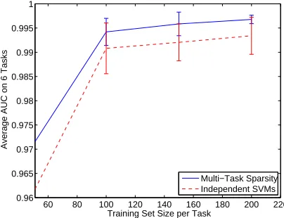
60 80 100 120 140 160 180 200 220 0.96

0.965 0.97 0.975 0.98 0.985 0.99 0.995 1

Training Set Size per Task

Average AUC on 6 Tasks

Multi−Task Sparsity Independent SVMs

Figure 1: Feature selection on the UCI Dermatology data set. Multitask sparse feature selection and independent SVM classification are compared. Various data set sizes are shown ranging from 20 to 200 samples for each of the 6 tasks. The average area under the ROC curve on test data is shown for all tasks for 5 folds (along with the standard deviation). The values

of C andαwere obtained by cross-validation on held out data.

progress requiring an unbounded number of iterations. We will show that is not the case and, indeed, the sequential quadratic programming procedure in Algorithm 1 will only require a finite number of iterations (of step 3). The number of iterations is bounded by Theorem 2 which is proved in the Appendix. It guarantees that, for anyα≥0,ε∈(0,1), Algorithm 1 finds a ˜λthat satisfies

J(_λ˜_{)≥(1−ε)J(λ}∗_)(whereλ∗_{is the constrained maximizer of J(λ)) in no more than}

&

log(1/ε)

log min 1+1

α,2

'

iterations. Here, each iteration involves (possibly warm-started) SVM programs and the expression

⌈. . .⌉denotes the integer ceiling function.

Therefore, a constant number of iterations is needed that depends only on α. In summary,

solving multitask feature or kernel selection is only a constant factor more computational effort than solving M independent support vector machines. A similar SQP or iterative SVM algorithm can be derived for the adaptive pooling setup described in Section 8.

11. Experiments

To evaluate the multitask learning framework, we considered UCI data8 as well as the Land Mine

data set9 which was developed and investigated in previous work (Xue et al., 2007). The

classi-fication accuracy of standard support vector machines learned independently is compared to the accuracy of the multitask kernel selection procedure described in Section 6 and Section 7. In all experiments, we explore multiple values of the regularizer C for the SVM and multiple values of

8. Data available athttp://archive.ics.uci.edu/ml/.