INTRODUCTION
The one of the applied branch of mathematics is Graph Theory. In the field of study there are a wide range of applications of graph theory the some of them are in operational research, genetics, physics, chemistry etc. Basically in the study of graph theory we can represent the relation ship between various objects in very simple and convenient way in the form of picture. For example in the field of chemistry if we want to represent chemical bonding between carbon atoms and the hydrogen atoms of C2H6 then with the help of graph we can easily represent this as follows
Basic Graphs Terminologies,
their Representation and Applications
VAIBHAV SHUKLA and SOMNATH GHOSH
Jagran Institute of Management 620, W Block Saket Nagar, Kanpur - 208 014 (India).
(Received: April 10, 2011; Accepted: May 15, 2011)
ABSTRACT
In the present study, general graph terminologies are explained with their representation and application in wide fields like operational research, genetics, physics and chemistry. Basically in the study of graph theory we can represent the relationship between various objects in very simple and convenient way in the form of picture.
Key words: Graphs, Genetics, Physics and Chemistry.
There are var ious other practical applications of graph theory which we used in our daily life for example we want to go from kanpur to mumbai and we dontknow the shor test route between the kanpur to mumbai then in this case there are various path for reaching from kanpur to mumbai for example as the graph shows we can go from kanpur to mumbai via delhi or via madras or we can go directly from kanpur to mumbai and the shortest distance coverd by this journey is to go directly from kanpur to mumbai so we can say that the convienent journey is to go directly from kanpur to mumbai hence we can say that if we have the graph then we can find out the shortest path between kanpur to mumbai and we use this path.
H H
H C C H
H H
The above figure shows the graph representation of the C2H6 and represent how the two molequels of carbon and the six hydrogen molequels are arranged.
Delhi 900km
Mumbai 600 km 600km 1100km
Kanpur
700 km
Chennai
Graph
edges and in this representation each edge joins exactly two vertices.
Definition
The mathematical definition of the graph shows that the graph is the collection of number of vertices and edges and in the graph there is set of vertices which is denoted by the V or V(G) and is called the vertex set of the graph G and there is a set of edges which is denoted by E or E(G) called the set of edges of graph G.Hence we can say that a graph G=(V,E) is the finite collection of vertices and edges where Vis the vertices or nodes of the graph G and E is the edges or line or link of the graph G.
Order of the Graph
The total no of vertices in the grph G is called the order of the graph G. It is also called the cardinality of the graph G and is represented by |V|.For example the vardinality or order of the graph 2 is seven because the total no of vertices in this graph is seven.
Size of graph
The total no of edges in the graph G is called the size of the graph G and is represented by |E|.For example in the graph 2 there are total of ten edges so the size of the graph g is ten.
called the parallel edges if these are associated with thee same vertex pair ,say,(Vi,Vj). In the graph-3 the edges e5 and e7 are the parallel edges which are associated with the same vertex pair (V4,V5)
Isolated Vertex
In a Graph a vertex with degree zero is called the isolated vertex or in other word we can say that the vertex which is not associated with any edge is called the isolated vertex. In the graph -3 the vertex V1 is called the isolated vertex.
Pendant Vertex
A vertex with degree one is called the pendent vertex of the graph G or in other world if there is only one edge associated with any vetex then the degree of that vertex is one and vertex is called the pendant vertex.In the graph -3 the vertex v7 is called the pendant vertex.
Degree of the Vertex
The total number of edges incident on a vertex is called the degree of that vertex. When we counted the degree of the vertex then the self loop is counted two times.
More Definitions Self Loop
An edge whose starting and ending point are same are called the self loop or we can say that the edge which is associated with the same vetex pair say (Vj,Vj) are called the self loop.In the graph-3 the edge e9 is the self loop whose starting and ending point is the vertex v6.
Parallel edge
The two ore more then two edges are
e3
v2 v3 e 8 e9
e e1 e2 e4 v6
v1
e 5 e 6
v7
·
e8 v4 v5
Fig. 3:
e 9
v2 v3 e 10
v4 e1 e2 Eeeeeeeeeeeeeee e4 v1
v5 e8 e5 v6 e6 e7
v7 e 3
Graph 2
In the above graph we calculate the degree of vertex as
follows-Deg(V1)=No of edges associated with the vertex V1=1(Because only edge e1 is associated with this vertex)
Deg(V4)=No of edges associated with the vertex V4=3(Because only edges e5 and e7are associated with this vertex)
Walk
In a Graph G=(V,E) where V is the set of vertices and E is the set of edges ,a finite alternative seequence of vertices and edges in such a way rhat each of the edge in the seequence is preeceded and followed bt the vertices and starting and ending point of the seequence are the verices are called the walk if in this seequence no edge appear more then once however the vertices may appear more than once.The starting and the ending vertices of the walk is called the terminal vertices.
If a walk begins and end with the same vertices then the walk is called an closed walk otherwise this walk is called open walk.
vertex appears more then once accept terminal vertices is called the circuit.
In the above Graph V1,e1,V2,e3,V3,e2,V1 is an cuircuit.
Types of Graph
In this heading we define the various types of graphs as
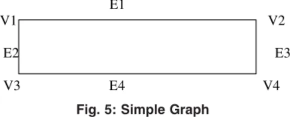
follows-Simple Graph
A graph G=(V,E) with vertex set V and edge set E is called a simple graph if it doesn’t contain any self loop and parallel edges.
V1 e2 e1
e V3
V2
e7
e4 e6 V6
V4 V5 e5
e8
e3
Fig. 4:
Now in the above figure V1,e2,V3,e6,V5,e5,V4,e4,V2 is an walk in the above graph similar to this walk we can find out many of the other walk say V1,e1,V2,e4,V4,e5,V5 is also an walk.
Path
In a Graph G an open walk is called an Path if in a walk no vertex appears more then once. Hence we can say that a path is a finite alternative seequence of vertices and edges in which no of the verices and edges appears more then once.The total number of edges in the path is called the length of the path.
In the above graph V1,e1,V2,e4,V4,e5,V5,e6,V3 is an path.
Cuicuit
In a graph G a closed walk in which no
E1
V1 V2
E2 E3
V3 E4 V4
Fig. 5: Simple Graph
In the above graph there is no any self loop and parallel edges so this is an Simple graph.
Finite and Infinite Graphs
A graph G=(V,E) with vertex set V and edge set E is called a Finite Graph if it contains finite number of vertices and edges and graph is a infinite graph if it has infinite number of vertices abd edges.
Fig.6 : (a)Finite Graph (b) Infinite Graph
In the above figures the graph (a) ccontains the finite no of vertices and edges so this is a finite graph and the graph (b) contains the infinite no of vertices and edges so this is called infinite graph
Null Graph
In this graph we have only finite set of vertex and the edge set is empty so this is called null graph.
Complete or Full graph
A graph without self loop and parallel edges is called a complete graph if there exist an edge between each and every pair of vertices.A complete graph of n vertices is denoted by Kn.
In the above graph we have only set of parallel edges so this is a multi graph.
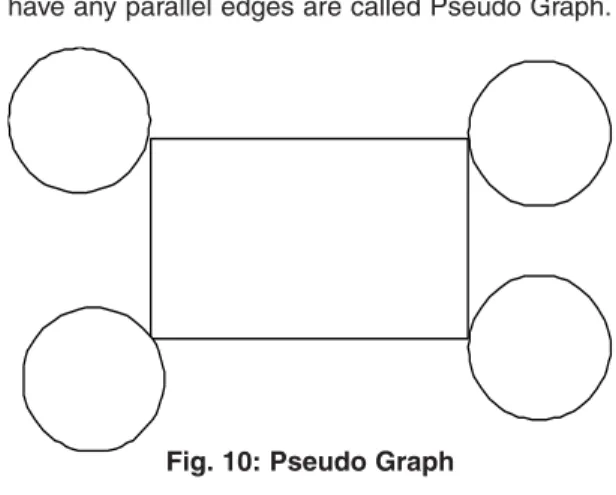
Pseudo Graph
A graph which contains self loops but don’t have any parallel edges are called Pseudo Graph.
·
·
·
·
Fig. 7: Null Graph
·
V1
E1 E2
V2
E3
Fig. 8: Complete graph
In the above graph there is no self loop and parellel edges and there is an edge between each and every pair of vertices.
Multi Graph
A graph which don’t have any self loops but must have some parallel edges are called the multi graph.
E3
V1 V2 E4
E1 E2 E5
V3 V4 E6
Fig. 9: Multi Graph
Fig. 10: Pseudo Graph
Regular Graph
A graph without self loops and parallel edges is called the regular graph if degree of each and every vertex are same in other world we can say that the simple graph in which the degree of all vertices are same is called the Regular Graph.
V1 E1 V2
E2 E4
V3 E3 V4
Fig. 11: Regular Graph
Here in the above graph the degree of all the vertices are same that is two hence this is a regular graph.
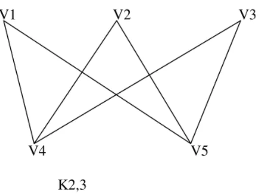
Bipartite Graph
A graph G=(V,E) are called the bipartite graph if the vertex set of the graph G is divided in to two non empty disjoint subsets V1(G) and V2(G) in such a way that each edge e of the graph g has its one end point in the vertex set V1(G) and the other end point is in the other vertex set say V2 (G)
V(G)={V1,V2,V3,V4,V5} in two par titions say {V1,V2,V3}and {V4,V5} and each of the vertex in one partition join with the vertex in the other partition.
Weighted Graph
The Graph G=(V,E) is called the weighted graph if the vertices or (and) edges contains some additional information such as assigning a positive number to the edges of G is called weighted graph. These numbers are called the weight of the edges.
The best examples of this graph is the railway tracks between different stations here the different cities shows the vertices of the graph G and the railway tracks are the edges of the graph. The edges in the graph has some additional information that is the distance between different cities.
Digraph or Directed Graph
A graph G=(V,E) is called the directed graph if in the graph there is an edge between the vertices Vi and Vj with an arrow directed from Vi to Vj.If the direction is from Vi toVj then Vi is the source for this edge and Vj is the sink of this edge.
V1 V2 V3
V4 V5
K2,3
Fig. 12: Bipartite Graph
V2 20 10
V1 V3 25
16 V4
Fig. 13: Weighted graph
Cycle Graph
A graph consist of n ver tices V1 ,V2,V3,………,Vn and edges (V1,V2),(V2,V3)(V3,V4)………..(Vn,V1) is called the cycle graph denoted by Cn. In a cycle graph there are equal no of vertices and edges.
V1
V2 V3
Fig. 14: Cycle Graph
V1 E1 V2 E2 E3
V3 E4 V4
E5
V5
Fig. 15: Directed Graph Planar Graph
A Graph G=(V,E) is called the planar graph if we can form some geometrical represeention of graph in such a way that no of the two edges of the graph crosses each other .
V1 V2
V3 V4
Fig. 16(a): Planar Graph V1 V2
In the Figure both the graph are the complete graph of four vertices but the graph (a) is a planar graph and the graph (b) is the non planar graph this shows that if we represent the graph (b) in such a way that the edges of the graph are not intersect each other is called planar graph.
Connected Graphs, Dissconected graphs and Components
If in a graph there exist a path betyween each and every pair of vertex then the graph is called the connected graph otherwise the graph is called the disconnected graph.
We can see that in a dissconnected graph there are two ore more connected graphs each of the graphs are the connected subgraphs of the graph G .So in adissconnected graph there are two or more connected subgraphs and each of the connected subgraph is called the components of the dissconnected graph.
In the above figure the figure 16(a) is the example of connected graph because in this graph there exist an path for each and every pair of vertices but the graph 16(b) is an example of the disconnected graph because there exist vertex pairs between which no path exist for example for vertex pair (V1,V5),(V2,V5) etc. are the vertex pair for
Fig. 17(b): Disconnected Graph
V4 V6
V3 V5
V1 V2
V1 V2 V3
V4 V5
Fig. 17(a): Connected graph
which no path exist hence this is a dissconnected graph.
Representation of the Graph
The graph can be reprented in many ways the some of them are disscussed here. The graph representation are applicable for both types of graph say directed and undirected graph hence we disscuss here both whenever applicable.
Adjacency Matrix
The adjacency matrix of the graph G with no parallel edges contains only binary elements say 0 and1.The elements of the adjacency matrix A are as follows
V1 E1 V2
E2 E3
V3 E4 V4
Fig. 18(a): Undirected Graph
The adjacency matrix for this graph is
V1 V2 V3 V4
V1 0 1 1 0
V2 1 0 0 1 A=
V3 1 0 0 1
V4 0 1 1 0
Fig. 18(b): Adjacency Matrix for graph 17(a)
V1 E1 V
E2
V3 E4
E5
V5
aij=1 If there is an edge between ith and jth vertices
= 0 If there is no edge between them
The examples shows the adjacency matrix for both directed and undirected graphs as follows
Properties
For an undirected graph with no parallel edges and self loop if we have the adjacency matrix then the degree of any vertex in the graph g is the number of 1 in the row or collum correspond to that vertex in the matrix.
The total number of non zero elements in the graph represents the number of edges in the graph.
Incidence Matrix
The entries of the incidence matrix of the Graph G=(V,E) where V is the set of vertices and E is the set of edges are
Aij = 1 if jth edge Ej is incident on the ith vertexVi
0 otherwise
This matrix is called the incident matrix or vertex edge matrix.
V1 V2 V3 V4 V5
V1 0 0 1 0 0
V2 1 0 0 1 0 A=
V3 0 0 0 1 1
V4 1 0 0 0 0
V5 0 0 0 0 0
Fig. 19(b): Adjacency matrix for figure 18(a)
a e1 b
e2 e5 ee c
e3 e e4 d
e8
f e6
e7
Fig. 20(a)
e1 e2 e3 e4 e5 e6 e7 e8 a 1 0 0 0 1 0 0 0
A=
b 1 1 0 0 0 1 1 0
c 0 1 1 0 0 0 0 0
d 0 0 1 1 0 0 1 0 e 0 0 0 1 1 1 0 1 f 0 0 0 0 0 0 0 1
Fig. 20(b): Incidence matrix of graph
Incident matrix For Directed Graph
Let G=(V,E) is an directed graph with no self loop then the entries of the incidence matrix for the directed graph are as follows
Aij= 1 if the jth edge is incident out of ith vertex -1 if the jth edge is incident in to ith vertex 0 if the jth edge is not incident on ith vertex
V2 V5
E2 E4 E5
E1
V3 E3 V4 V6
V1
E6 E8 E9
E7
V8 V7
Fig. 21(a):
E1 E2 E3 E4 E5 E6 E7 E8 E9
V1 1 0 0 0 0 1 0 0 0
V2 -1 1 0 0 0 0 0 0 0 A=
V3 0 -1 1 0 0 0 -1 0 0
V4 0 0 -1 1 0 0 0 -1 0
V5 0 0 0 -1 -1 0 0 0 0
V6 0 0 0 0 1 0 0 0 -1
V7 0 0 0 0 0 0 0 -1 -1
Fig. 21(b): Incident Matrix For graph 20(a)
Linked List Representation Of Graph
V1 Null
V2 Null
V3 Null
V4 Null
V5 Null
V6 Null
V7 Null
V8 Null
V9 Null
V2 V1
V8 V2 V2 V3 V5
V6 V5
V7 V8 V8 V4 V5 V5 V3
V7 V6
V4
V3 V9 V1
V5
V8 V2
V4 V7
Fig. 22(a)
Fig. 22(b) Linked List Representation Of Graph 21(a)
Colouring of the Graph
In the colouring of the Graph we colour all the vertices of the graph G in such a way that no two of the adjacent vertices have the same colour.A graph in which every vertex is painted according to the proper colouring then the graph is called a properly coloured graph.
In the above Graph we want to colour the all the vertices pof the graph G in such a way that no two adjacent vertices have the same colour so first we assign the colour red to vertex V1 now the other two vertices are adjacent to the vertices V1 hence we can not assign colour red to vertices V2 and V3 so we assign the colour green to the vertex V2 at last vertex V3 are adjacent to the vertex V1 and V2 so we can not assign colour red and green to V3 so we assign colour Bblack to V3. The three colours are required for the proper colouring of this graph the total number of colours requiered for the proper colouring of the graph G is called the chromatic number of that graph. So the chromatic number of the above graph is three.
V1
V2 V3
1. Berge, Claude (1958), Théorie des graphes et ses applications, Collection Universitaire de Mathématiques, II, Paris: Dunod . English edition, Wiley 1961; Methuen & Co, New York 1962; Russian, Moscow 1961; Spanish, Mexico 1962; Roumanian, Bucharest 1969; Chinese, Shanghai 1963; Second printing of the 1962 first English edition, Dover, New York 2001.
2. Biggs, N.; Lloyd, E.; Wilson, R., Graph
Theory, 1736–1936, Oxford University
REFFERNCES
Press (1986).
3. Bondy, J.A.; Murty, U.S.R., Graph Theory,
Springer (2008)
4. Chartrand, Gary, Introductory Graph Theory,
Dover, ISBN 0-486-24775-9 (1985).
5. Gibbons, Alan, Algorithmic Graph Theory,
Cambridge University Press (1985).
6. Golumbic, Martin, Algorithmic Graph Theory
and Perfect Graphs, Academic Press (1980).
7. Harary, Frank, Graph Theory, Reading, MA: