http://www.sciencepublishinggroup.com/j/pamj doi: 10.11648/j.pamj.20170601.17
ISSN: 2326-9790 (Print); ISSN: 2326-9812 (Online)
Cubic B-spline Collocation Method for One-Dimensional
Heat Equation
Mohamed Hassan Khabir
1, Rahma Abdullah Farah
21Department of Mathematics, Faculty of Science, Sudan University of Science & Technology, Khartoum, Sudan 2
Department of Mathematics, Faculty of Science & Technology, Omdurman Islamic University, Khartoum, Sudan
Email address:
[email protected] (M. H. Khabir), [email protected] (R. A. Farah)
To cite this article:
Mohamed Hassan Khabir, Rahma Abdullah Farah. Cubic B-Spline Collocation Method for One-Dimensional Heat Equation. Pure and Applied Mathematics Journal. Vol. 6, No. 1, 2017, pp. 51-58. doi: 10.11648/j.pamj.20170601.17
Received: November 26, 2016; Accepted: January 16, 2017; Published: March 4, 2017
Abstract:
In this paper we discuss cubic B-spline collocation method. We have given the derivation of the B-spline method in general. We have applied the method for solving one-dimensional heat equation and the numerical result have been compared with the exact solution.Keywords:
Cubic B-spline, Collocation Method, Heat Equation, Linear Partial Differential Equation1. Introduction
Consider the one dimensional initial-boundary value problem
= 0, = 0, 1, = 0 .= , = 1 , 0 = g .
(1)
This problem is one of the well-known second order parabolic linear partial differential equation [1, 3, 4]. The heat equation is a very important equation in physics and engineering. It shows that heat equation describes the distribution of heat (or variation in temperature) in a given region over time. The heat equation is of fundamental importance in diverse scientific fields. In mathematics, it is prototypical parabolic partial differential equation. In probability theory, the heat equation is connected with the study of Brownian motion via the Fokker – Planck equation [5]. Numerical solutions of those equations are very useful to study physical phenomena. One of the linear evolution equation which we deal with the numerical solution is the heat equation [2]. In financial mathematics it is used to solve the Black – Scholes partial differential equation. The diffusion equation, a more general version of the heat equation, arises in connection with the study of chemical diffusion and other related processes [5]. In history, the heat
1995). An abstract form of heat equation on manifolds provides a major approach to the Atiyah – Singer index theorem, and has led to much further work on heat equations in Riemannian geometry [5].
In this study the cubic B-spline collocation method is used [7, 9, 10] for solving the heat equation (1) and the solutions are compared with the exact solution. In the section two, we have given the derivation for the B-spline method and uniform convergence for the method has been
discussed. Finally, we have solved the problem (1) using the method, the numerical results and graphs have also been shown.
2. B-spline Collocation Method
We define the cubic B-spline for = 0,1,2, … , .
=
! "# $ %&
'( ) *
, if ∈ . $/, $01,
1 + 3 # $ %&4
'( ) + 3 # $ %&4
'( ) /
+ # $%&4
'( ) *
, if ∈ . $0, 1,
1 + 3 # %54$
'( ) + 3 # %54 $ '( )
/
+ # %54$
'( ) *
, if ∈ . , 601,
# %5 $
'( ) *
, if ∈ . 60, 6/1,
0, otherwise,
(2)
where ℎ? = 60− , = −1,0, … , + 1.
We introduce four additional knots as $/< $0< B and
C6/> C60> C.
From the above Eq. (2) we can simply check that each of the functions is twice continuously differentiable on the entire real line, also
E FG = H
4, if = J, 1, if − J = ±1,
0, if − J = ±2, (3)
and that = 0 for ≥ 6/ and ≤ $/. Similarly we can show that
Q
R = H
0, if = J, ±*'(, if − J = ±1, 0, if − J = ±2,
(4)
and
QQE FG =
−'(0/, if = J,
S
'( , if − J = ±1,
0, if − J = ±2.
(5)
Each is also a piece-wise cubic with knots at T, and
∈ U.
The values of , Q and QQ at the nodal points
′W are shown in Table 1.
Table 1. B-Spline basis values.
Nodal values
Let Ω = Y $0, B, 0, … , C60Z and let [* T = span Ω. The functions Ω are linearly independent on .0,11, thus
[* T is + 3 -dimensional. Even one can show that
[* T ⊆^_U. Let ` be a linear operator with domain U and with range in U.
Now we define
= ∑C60b$0 = $0 $0 + B B + 0 0 +
⋯ + C C + C60 C60 . (6)
Then force ) to satisfy the collocation equations plus the boundary conditions.
We have
`0 E FG = dE FG 0 ≤ F ≤ N, (7)
and
0 = fB, 1 = f0. (8)
On solving Eq. (7), we get
−g QQ
F + hE FG F = d F
⇒ −g j QQE
FG + hE FG j E FG C60
b$0 C60
b$0
= d F
⟹ −g l F$0 F$0QQ E FG + F FQQE FG + F60 F60QQ F m
+ h F lF$0 F$0E FG + F FE FG
+ F60 F60 F m = d F ∀J = 0,1, … , ,
⟹ F$0l−g F$0QQ EFG + hF F$0E FGm + Fl−g FQQEFG +
hF FE FGm + F60l −g F60QQ E FG + hF F60E FG m = dF ∀J =
0,1,2, … , , (9)
by using equations (3) and (5) we get
E−6g + hFh?/GF$0+ E12g + 4hFh?/GF+ E−6g +
hFh?/GF60= h?/dF, ∀J = 0,1, … , , (10)
where hE FG = hF and dE FG = dF. The given boundary conditions (8) become
x xi-2 xi-1 xi xi+1 xi+2
0 1 4 1
ℎ? Q 0 −3 0 3 0
F = B = fB
⟹ $0 $0 B + B B B + 0 0 B + ⋯
+ C60 C60 B = fB
⟹ $0+ 4 B+ 0= fB, (11)
and
F = C = f0
⟹ $0 $0 C + B B C + 0 0 C + ⋯
+ C$0 C$0 C + C C C
+ C60 C60 C = f0
⟹ C$0+ 4 C+ C60b f0. (12)
Eqs. (10), (11) and (12) lead to a + 3 × + 3 tridiagonal system with + 3 unknowns C=
$0, B, … , C60 (where t stands for transpose).
Now eliminating $0 from the first equation of (10) and (11), we find
36g B= dBh?/− fBE−6g + hBh?/G. (13)
Similarly, eliminating C60 from the last equation of (10) and from (12), we find
36g C= dCh?/− f0E−6g + hCh?/G. (14) from (10) we get
J = 1: −6g + h0 h?/ B+ E12g + 4h0h?/G 0+ E−6g + h0h?/G /= Z0h?/
J = 2: −6g + h/h?/ 0+ E12g + 4h/h?/G /+ E−6g + h/h?/G *= Z/h?/ ⋮
J = : −6g + h h?/
$0+ E12g + 4h h?/G + E−6g + h h?/G 60= Z h?/
⋮
J = − 1: E−6g + hC$0h?/G C$/+ E12g + 4hC$0h?/G C$0+ E−6g + hC$0h?/G C = Zt$0h?/.
The above equations lead to the system of + 1 linear equations u C = vC in the + 1 unknowns C= B, … , C of the form
w x x x x
y36gz { z z { z
⋱ ⋱ ⋱
z { z
36g}~ ~ ~ ~ •
w x x x x y B0
/
⋮
C$0 C }
~ ~ ~ ~ •
=
w x x x x x
ydBh?/− fBz
d0h?/
d/h?/
⋮ dC$0h?/
dCh?/− f0z}
~ ~ ~ ~ ~ •
, (15)
where
z = −6g + hh?/,
{ = 12g + 4hh?/.
Since h > 0, it is easily seen that the matrix u is strictly diagonally dominant and hence nonsingular. Since u is nonsingular, we can solve the system u C= vC for
B, 0, … , C and substitute into the boundary equations (11) and (12) to obtain $0 and C60
Lemma [8] The B-splines Y $0, B, … , C60Z defined in equation (2), satisfy the inequality
j |B | ≤ 10,
t60
‚b$0
0 ≤ ≤ 1.
Proof. We know that
ƒ j B
C60
b$0
ƒ ≤ j | |
C60
b$0
.
At any th nodal point we have
j |B | = |B$0| + |B | + |B60| = 6 < 10 t60
b$0
.
Also we have
| | ≤ 4 and | $0 | ≤ 4 for ∈ . $0, 1.
Similarly
| $/ | ≤ 1 and | 60 | ≤ 1 for ∈ . $0, 1.
Now for any point ∈ . $0, 1 we have
j | | = | $/| + | $0| + | | + | 60| ≤ 10. C60
b$0
Hence this proves the lemma.
3. Numerical Result
, = „$…† sin 2T , g = sin 2T .
Denote the value of at the representative mesh point
E F, ‡G by
ˆ= E F, ‡G = F‡
The forward difference approximation for is
≈ Š‹54$ Š‹
∆ (16)
Substitute = F in (16) we get
‡60 − ‡
∆ = •
/
• / ‡60
⟹ −∆ ‡60+ ‡60= ‡
At = 0: Ž = 0 ⟹ B
−∆ 0 + 0= B (17)
⟹ −g•QQ+ • = g
Substitute
0 = j QQ F C60
b$0
, 0= j E FG, C60
b$0
B= E F, 0G
= gE FG, ∆ = •
in (17) we get
−• j QQ
F C60
b$0
+ j F
C60
b$0
= g F
⟹ −• l F$0 F$0QQ E FG + F FQQE FG + F60 F60QQ F m + F$0 F$0E FG + F FE FG + F60 F60 F = g F ∀J = 0,1, … , ,
⟹ F$0l−• F$0QQ E FG + F$0E FGm + Fl−• FQQE FG + FE FGm + F60l−• F60QQ E FG + F60 F m = gE FG∀J = 0,1, … , , (18)
by using equations (3) and (5) we get
E−6• + h?/G
F$0+ E12• + 4h?/GF+ E−6• + h?/GF60= gFh?/ ∀j = 0,1, … , N, (19)
J = 1: −6• + h?/
B+ E12• + 4h?/G 0+ E−6• + h?/G /= g0h?/
J = 2: −6• + h?/ 0+ E12• + 4h?/G /+ E−6• + h?/G *= g/h?/
⋮
J = : −6• + h?/ $0+ E12• + 4h?/G + E−6• + h?/G 60
= g h?/
⋮ J = − 1: E−6• + h?/G
C$/+ E12• + 4h?/G C$0
+ E−6• + h?/G C= gt$0h?/.
The above equations lead to the system of + 1 linear equations u C= vC in the + 1 unknowns C =
B, 0, … , C of the form
w x x x x
y36•z { z z { z
⋱ ⋱ ⋱
z { z
36•}~ ~ ~ ~ • w x x x x y B0
/ ⋮ C$0 C } ~ ~ ~ ~ • = w x x x x x y gBh?/
g0h?/
g/h?/
⋮ gt$0h?/
gCh?/ }
~ ~ ~ ~ ~ •
, (20)
where
z = −6• + h?/,
{ = 12• + 4h?/.
We can see that the system is strictly diagonally dominant and hence nonsingular. So we can solve the system for
B, 0, … , C and substitute into the boundary conditions (11)
and (12) to obtain $0 and C60.
The table 2 below illustrates the numerical, exact solution and error for the heat equation
Table 2. Numerical, Exact Solution And Error For The Heat Equation .
x p_i Numerical U_exact error
0 0 0 0
0.0500 0.0108 0.0060 0.0185
0.1000 0.0206 0.0113 0.0353
0.1500 0.0284 0.0156 0.0486
0.2000 0.0333 0.0184 0.0571
0.2500 0.0351 0.0193 0.0600
0.3000 0.0333 0.0184 0.0571
0.3500 0.0284 0.0156 0.0486
0.4000 0.0206 0.0113 0.0353
0.4500 0.0108 0.0060 0.0185
0.5000 0.0000 0.0000 0.0000
0.5500 -0.0108 -0.0060 0.0185
0.6000 -0.0206 -0.0113 0.0353
0.6500 -0.0284 -0.0156 0.0486
0.7000 -0.0333 -0.0184 0.0571
0.7500 -0.0351 -0.0193 0.0600
0.8000 -0.0333 -0.0184 0.0571
0.8500 -0.0284 -0.0156 0.0486
0.9000 -0.0206 -0.0113 0.0353
0.9500 -0.0108 -0.0060 0.0185
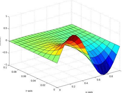
Figure 1. Exact solution for the heat problem .
Figure 2. Numerical solution for the heat problem using ℎ = 0.05 and • = 0.01. 0
0.2
0.4
0.6
0.8
1
0 0.02 0.04 0.06 0.08 0.1
−1 −0.5 0 0.5 1
x−axis t−axis
Solution
0
0.2
0.4
0.6
0.8
1
0 0.02 0.04 0.06 0.08 0.1
−1 −0.5 0 0.5 1
x−axis t−axis
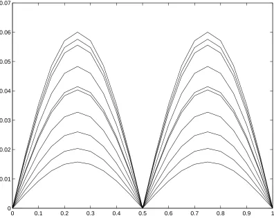
Figure 3. This shows the error for the heat problem using ℎ = 0.05 and • = 0.01.
Figure 4. This shows the error for the heat problem using ℎ = 0.01 and • = 0.001.
0 0.1 0.2 0.3 0.4 0.5 0.6 0.7 0.8 0.9 1
0 0.01 0.02 0.03 0.04 0.05 0.06 0.07
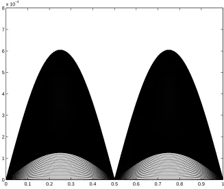
0 0.1 0.2 0.3 0.4 0.5 0.6 0.7 0.8 0.9 1
0 1 2 3 4 5 6 7 8x 10
Figure 5. This shows the error for the heat problem using ℎ = 0.01 and • = 0.0001.
4. Conclusion
We applied the cubic B-spline collocation method to solve one-dimensional heat equation. The results and graphs have also been shown using MATLAB for the comparison between the numerical and exact solutions.
Numerical experiments are conducted to demonstrate the viability and the efficiency of the proposed method computationally.
Appendix
Program for the heat problem : Main_bspline:
clc clear
h = 0.05; x0 = 0; x1 = 1; b = 1; t0 = 0; t1 = 0.1; k = 0.01; % h = 0.05; x0 = 0; x1 = 1; b = 1; t0 = 0; t1 = 0.1; k = 0.001;
% h = 0.01; x0 = 0; x1 = 1; b = 1; t0 = 0; t1 = 0.1; k = 0.001;
% h = 0.01; x0 = 0; x1 = 1; b = 1; t0 = 0; t1 = 0.1; k = 0.0001;
% j = 0;1;...;n; x = x0: h: x1; sizex = x; t = t0: k: t1; M = length(x); N = length(t); p0 = sin(2*pi*x); u = zeros(N,M); u(1,:) = p0;
% M = M - 2; for i = 2: N
[p_i] = fun_bspline(p0,h,k,M); u(i,:) = p_i;
p0 = p_i; end
%%%%%%%%%%%%%%%%%%%%%%%%%%%% %%%%%
V = zeros(N,M); V(1,:) = sin(2*pi*x); for i = 1: N
for j = 1: M
V(i,j) = exp(-4*t(i)*pi^2)*sin(2*pi*x(j)); U_exact(j) = exp(-4*t(i)*pi^2)*sin(2*pi*x(j)); end
end
error = max(abs(u – V)); yerr = abs(u-V);
y=[x' p_i' U_exact' error'] %---
Figure(1) surf(x,t,V) %--- % figure(1) % plot(x,yerr) %--- figure(2) surf(x,t,u) %---
%%%%%%%%%%%%%%%%%%%%%%%%%%%% %%%%%%%
%
0 0.1 0.2 0.3 0.4 0.5 0.6 0.7 0.8 0.9 1
0 1 2 3 4 5 6 7 8x 10
% surf(x,t,u) Fun_bspline:
function YYp = fun_bspline( p0,h,k,M) gammaj = 12*k + 4*h^2;
alphaj = -6*k + h^2; betaj = -6*k + h^2; A = zeros(M,M); Mvalue = M;
A = diag([36*k ones(1,M-2)*gammaj 36*k],0 +… diag([0 ones(1,M-2)*alphaj],1) +…
diag([ones(1,M-2)*betaj 0],-1); ft = p0;
alpha0 = 0; alpha1 = 0; yp0 = alpha0; yp1 = alpha1; dm = h^2*ft;
dm(1) = dm(1) - yp0*(-6*k+h^2); dm(M) = dm(M) - yp1*(-6*k+h^2); Amatrix = A;
dm = dm'; sizeA = size(A); sizedm = size(dm); cc = A\dm;
ccm1 = 0 - 4*cc(1) - cc(2); ccmp1 = 0 - 4*cc(M) - cc(M-1); ccc = [ccm1 cc' ccmp1];
YYp = ccc(1:M) + 4*ccc(2:M+1) + ccc(3:M+2); end
References
[1] H. S. Carslaw, J. C. Jaeger, Conduction of Heat in Solids, Oxford University Pres., 1959.
[2] I. Dag, B. Saka, D. Irk, Application Cubic B-splines for Numerical Solution of the RLW Equation, Appl. Maths. and Comp., 159 (2004) 373–389.
[3] D. V. Widder, The Heat Equation, Academic Press, 1976. [4] J. R. Cannon, The One-Dimensional Heat Equation,
Cambridge University Pres., 1984. [5] en.wikipedia.org/wiki/Heat_equation.
[6] JBJ Fourier, Theorie analytique dela Chaleur, Didot Paris: 499-508 (1822).
[7] J. M. Ahlberg, E. N. Nilson, J. L. Walsh, The Theory of splines and Their Applications, Academic Press, New York, 1967.
[8] M. K. Kadalbajoo and V. K. Aggarwal, Fitted mesh B-spline collocation method for solving self-adjoint singularly perturbed boundary value problems, AppliedMathematics and Computation 161 (2005), 973–987.
[9] G. Micula, Handbook of Splines, Kluwer Academic Publishers, Dordrecht, The Netherlands, 1999.