J.-S. Dhersin, Editor
SHAPE DEFORMATION AND OPTIMAL CONTROL
Sylvain Arguill`
ere
1, Emmanuel Tr´
elat
2, Alain Trouv´
e
3and Laurent Youn`
es
4Abstract. Shape deformation analysis is concerned with determining a deformation of a given shape into another one, which is optimal for a certain cost. We provide the main ideas for a new general approach to shape deformation analysis, using the framework of optimal control theory.
This point of view can be made independent from the parametrization of the shape, and allows to model general constrained shape analysis problems. The use of a infinite dimensional variant of the con-strained Pontryagin Maximum Principle characterizes the optimal solutions of the shape deformation problem in a very general way.
R´esum´e. L’analyse des d´eformations consiste `a d´eterminer une transformation d’une forme donn´ee en une autre, optimale pour un certain coˆut. Nous donnons ici les id´ees principales pour une nouvelle approche g´en´erale pour cette analyse `a l’aide de la th´eorie du contrˆole optimal.
Ce point de vue peut ˆetre pris de mani`ere `a ne pas d´ependre de la param´etrisation de la forme, et permet ´egalement de mod´eliser des contraintes dans les probl`emes d’analyse de d´eformations. Nous utilisons une variante en dimension infinie (cadre naturel de l’analyse des d´eformations) du principe du maximum de Pontryagin avec contraintes permettant de caract´eriser de fa¸con tr`es g´en´erale les d´eformations optimales recherch´ees.
Introduction
The mathematical analysis of shapes has become a subject of growing interest in the past few decades, and has motivated the development of efficient image acquisition and segmentation methods, with applications to many domains, including computational anatomy and object recognition.
The general purpose of shape analysis is to compare two (or more) shapes embedded in a space IRdin a way that takes into account their geometric properties, or how ”similar” they look. InShape deformation analysis, a cost for every possible deformation of a shape is considered, and the problem is to find the deformation which minimizes this cost.
Taking a hint from fluid dynamics, we will consider deformations given by flows of diffeomorphisms generated by time-dependent vector fields (see [6, 15, 16]): deformations of the whole space, like diffeomorphisms, induce deformations of the shape itself.
1Universit´e Pierre et Marie Curie (Univ. Paris 6), CNRS UMR 7598, Laboratoire Jacques-Louis Lions, F-75005, Paris, France
2 Universit´e Pierre et Marie Curie (Univ. Paris 6) and Institut Universitaire de France and Team GECO Inria Saclay, CNRS
UMR 7598, Laboratoire Jacques-Louis Lions, F-75005, Paris, France ([email protected]).
3Ecole Normale Sup´erieure de Cachan, Centre de Math´ematiques et Leurs Applications, CMLA, 61 av. du Pdt Wilson, F-94235
Cachan Cedex, France ([email protected]).
4Johns Hopkins University, Center for Imaging Science, Department of Applied Mathematics and Statistics, Clark 324C, 3400
N. Charles st. Baltimore, MD 21218, USA ([email protected]).
c
EDP Sciences, SMAI 2014
This framework has led to the development of a family of registration algorithms called Large Deformation Diffeomorphic Metric Mapping (LDDMM), in which the correspondence between two shapes comes from the minimization of an objective functional that is the sum of two terms (see [4, 5, 9, 11, 12]). The first term is the total kinetic energy of the deformation (the L2-norm of the vector field in the case of fluid dynamics, though
ours will usually be different). The second term is a data attachment penalizing the difference between the deformed shape and a target.
This framework allows one to use tools from Riemannian geometry (see [17]), along with classical results from the theory of Lie groups equipped with right-invariant metrics (see [2, 3, 8, 10, 18]). However, our approach uses control theory, in particularoptimal control (see preliminary ideas in [17]).
While accounting for some of the geometric information in the shape, like singularities, it does not consider other intrinsic properties of the studied shape, which can also depend on the nature of the object modeled by the shape: one may wish the total volume of the shape to remain constant (water balloon), or the movement to occur only along certain directions (fibers in a muscle). It is therefore important to be able to add constraints to the problem.
The purpose of this paper is to summarize and report on the authors’s results in [1]. Since shape analysis has a natural setting in infinite dimension (indeed, the shape space is typically the space of all submanifolds in IRd), we will need to derive an appropriate infinite dimensional variant of the Pontryagin Maximum Principle (or PMP) with an infinite number of equality constraints.
1.
The point of view of optimal control for shape deformation
In this paper, ashape space M is a space of continuous maps from a smooth compact Riemannian manifold S into an Eucliddean space IRd. The elements of M are states of the shape, denoted by q : S → IRd. For example, ifS is the unit circle then M is the set of all parametrized continuous closed curves in IRd. WhenS has dimension 0, it is a finite union of points{s1, . . . , sn}. In this case,M = (IRd)nis finite dimensional. This is
the most important case for practical applications, and it is frequently used to approximate infinite dimensional problems.
Deformation through the group action of diffeomorphisms.The group of diffeomorphisms has a left action on the shape space by composition: forϕ∈Diff(IRd) andq∈M =C0(S,IRd
), we haveϕ·q=ϕ◦q.The mapq7→ϕ·q is of classC` wheneverϕis of classC`.
A deformation of IRd is a one-parameter family of diffeomorphisms (ϕ(t))t∈[0,1] with ϕ(0) =IdIRd. Such a
deformation produces adeformation q: [0,1]→M of an initial shapeq0 by lettingq(t) =ϕ(t)◦q0.
A classical problem of shape deformation is to find an ”optimal” deformation of an initial state q0 into a
final state close to a targetq1. More precisely, we will want to minimize a function of the formE(ϕ) +g(q(1)),
over all deformations ϕ= (ϕ(t))t∈[0,1] of IR d
. Here, E is a functionnal representing the kinetic energy of the deformation,q(1) =ϕ(1)◦q0 is the final state, andg is a data attachment measuring how close the final state
is from the targetq1. To defineE, we take a hint from fluid mechanics and use Euler-Lagrange coordinates.
Induced control system.Letvbe a bounded vector field of classC1. Theinfinitesimal actionofvon a state q∈M, denotedξqv, is defined as the composition ξqv =v◦q. It is also the velocity vector at 0 of the curve t7→ϕv(t)·q, whereϕv(t,·) is the flow ofv.
Example 1. An interesting case is whenS= (s1, . . . , sn) is a zero-dimensional manifold and M = Lmkd(n) = (IRd)n
is the (so-called) space ofnlandmarks in IRd. Forq= (x1, . . . , xn), the action of a diffeomorphismϕ is given
byϕ·q= (ϕ(x1), . . . , ϕ(xn)). For a bounded vector fieldv of classC1 on IRd, the infinitesimal action ofv atq
Most deformations can be ”parametrized” as flows of time-dependent vector fields
v= (v(t))t∈[0,1].
Moreover, ifϕis the flow associated to v, we get
˙ q(t) = d
dt(ϕ(t)◦q0) =v(t)◦(ϕ(t)·q0) =v(t)◦q(t).
Therefore, we get the following control system onM
q(0) =q0, q˙(t) =v(t)◦q(t), a.e. t∈[0,1].
Usually, one takesv to be at least inL1([0,1],C1
b([0,1],IR d
)), i.e. time-dependent bounded vector fields of class C1, integrable with respect to time, which ensures the existence of a flow.
The energy E of a deformation can then be defined directly on the control. For this, we restrict ourselves to vector fields belonging to some Hilbert spaceV of bounded vector fields of classC1, such as a Sobolev space Hk(IRd,IRd) withkbig enough. The total energy of a time-dependent vector field vis then defined by
E(v) =
Z 1
0
kv(t)k2dt.
Remark 1. It is possible to take more general energy, though one usually focuses on positive definite bilinear forms.
Mixed constraints can then be added to this system, defined by someC :M ×V →Y, Y a Banach space. We will only consider constraints linear with respect to the control (i.e. v). We will denoteC(q, v) =Cqv to
emphasize this last point.
We finally get our optimal control formulation of the shape deformation problem.
Problem 1. Let q0 ∈M, and let C :M ×V →Y be a mapping such that v 7→ C(q, v) =Cqv is linear for
every q∈M. Let g:M →IR be a function. We consider the problem of minimizing the functional
J1(v) =
1 2
Z 1
0
kv(t)k2Vdt+g(q(1))
over all time-dependent vector fields v(·) ∈ L2(0,1;V) such that C
q(t)v(t) = 0 for every t ∈ [0,1], where q(·) : [0,1]→M is the curve defined byq(0) =q0 andq˙(t) =ξq(t)v(t) for almost everyt∈[0,1].
Remark 2. The problem could be posed for more general (i.e. non-linear) constraintsC(q, v) = 0. We focused on linear constraints because such constraints often have a clearer geometric meaning.
2.
Existence and properties of optimal controls
In this section, we give sufficient conditions for the existence of a solution to Problem 1, and first-order necessary conditions for optimality, on the basis of the well-known Pontryagin Maximum Principle (PMP, see [7,13]) in optimal control theory. The extension to our infinite dimensional framework is however nontrivial. This allows us to derive the constrained geodesic equations for shape spaces.
Throughout the section, we adopt the framework and the notations defined in Section 1. LetM be the shape space of a compact smooth Riemannian manifoldS. LetV be a Hilbert space of bounded vector fields of class C1 on IRd
, and Y be a Banach space. Let C:M×V →Y be a mapping such that v7→C(q, v) =Cqvis linear
Existence of an optimal control. Our first theorem establishes the existence of solutions to Problem 1 under minimal assumptions.
Theorem 1. Ifq7→Cq andg are continuous, if g is bounded from below, and if V has a continuous inclusion
in the space of C1 bounded vector fieldswith bounded derivatives, then Problem 1 has at least one solution.
This is a consequence of Ascoli’s Theorem, combined with the usual proof for the existence of optimal control in finite dimensions (see [14]).
First-order optimality conditions. In this section, we state first-order necessary conditions for optimality in Problem 1 by extending the Pontryagin Maximum Principle to our setting.
For this, we need to define the hamiltonianH :M ×M∗×V ×Y∗→IR of the problem by
H(q, p, v, λ) =hp, ξqviM∗,M−
1 2kvk
2
V − hλ, CqviY∗,Y.
Theorem 2. Assume that g and C are of class C1, and thatV has a continuous inclusion in the space of C1
bounded vector fieldswith bounded derivatives.
If v 7→ Cqv is surjective for all q ∈ M, then for any optimal control v ∈ L2(0,1;V), there exist p ∈ H1(0,1;M∗)andλ∈L2(0,1;Y∗) such thatp(1) +dgq(1)= 0 and
˙
q(t) = ∂pH(q(t), p(t), v(t), λ(t)),
˙
p(t) = −∂qH(q(t), p(t), v(t), λ(t)),
0 = ∂vH(q(t), p(t), v(t), λ(t)),
for almost everyt∈[0,1].
The proof follows from the application of the infinite dimensional constrained extremum theorem combined with a careful analysis of the Lagrange multipliers.
Remark 3. The theorem should hold true for non-linear equality constraintsC(q, v) = 0, with the assumption that ∂vCq,v is surjective for every (q, v)∈M ×V, but one must then consider controls inL∞(0,1;V) instead
ofL2.
Remark 4. Note that the surjectivity assumption is a strong one in infinite dimension. It is usually not satisfied in the case of shape spaces whenY is infinite dimensional.
Remark 5. This is a ”weak” maximum principle: we derive the condition∂vH= 0 along any extremal, instead
of the usual (stronger) maximization condition. However, in the case of shape spaces,v7→H(q, p, v, λ) is strictly concave and hence both conditions are equivalent.
Remark 6. Taking the energy to be the L2-norm on vector fields of IRd instead of the norm on V, letting Cqv= divv, and applying the theorem gives the usual incompressible Euler equations of fluid mechanics (see [2]).
The Geodesic Equations on a Shape Space. A careful analysis of the equations of the PMP allows us to expressv andλas functions ofqandp, with
vq,p=KV ξq∗p−C ∗ qλ
and
λq,p=λq,p= (CqKVCq∗) −1C
qKVξ∗qp.
This allows us to define the reduced Hamiltonianh:M×M∗→IR as
h(q, p) =H(q, p, vq,p, λq,p),
and prove that optimal trajectories satisfy the usual Hamiltonian equations [3].
Proposition 1. (Geodesic Equations in Shape Spaces) If the assumptions of Theorem 2 are satisfied, then for any trajectoryq: [0,1]→M of a solution v of Problem 1, there is a map p∈H1(0,1;M∗)such that p(1) +dgq(1)= 0 and for a.e. t∈[0,1]and(q, p)satisfies the equations
(
˙
q(t) =∂ph(q(t), p(t)),
˙
p(t) =−∂qh(q(t), p(t)).
(1)
Such a couple(q, p)is called a geodesic. Moreover,t7→ 1 2kv(t)k
2 is constant. In particular, the total cost J 1(v)
of the trajectory is given by
J1(v) =
1 2kv(0)k
2
V +g(q(1)).
This gives a minimization algorithm, called minimization by shooting. Indeed, assume thatC and all vector fields in V are of class C2. Then an initial momentum p
0 ∈M∗ gives a unique geodesic (q, p) from the initial
stateq0. Now, ifqis an optimal trajectory if and only if it minimizes the reduced cost
J2(p0) =
1
2kvq0,p0k
2
V +g(q(1)).
This can be done using a gradient descent for a particular inner product.
3.
Examples of Matching
Constant Total Volume.For our first example, we consider a very simple constraint. Consider S =S1 the
unit circle in IR2, and let M =C1(S,IRd
) be our shape space. Note that we took a smaller shape space here, but our results still work, although with slightly stronger hypotheses (mainly,V must have bounded derivatives of order 2 for theorems 1 and 2, and bounded derivatives of order 3 for existence and unicity of solutions to the geodesic equations).
Assume the initial stateq0(s) = (x(s), y(s)) is a simple closed curve of class C1. This property is conserved
through deformation by diffeomorphism.
Such a curve is the boundary of an open subsetU(q) with total area given byV ol(U(q)) =R
Sx(s)dy(s).Now,
define a targetq1 such that V ol(U(q0)) =V ol(U(q1)). We take the constraintsV ol(U(q(t))) =V ol(U(q0)) for
every t∈[0,1].
We will considerV, a reproducing kernel Hilbert space of smooth vector fields given by the Gaussian kernel with positive scaleσ(see [17] for definitions).
For numerical applications, we will taked= 2, soS=S1andM is a space of curves, which will be discretized
as landmarks q= (x1, . . . , xn) ∈Lmk2(n). In this case, the volume of a curve is approximately equal to the
volume of the polygonP(q) with vertices (xi), given by
V ol(P(q)) = 1
2(x1y2−y2x1+· · ·+xny1−ynx1).
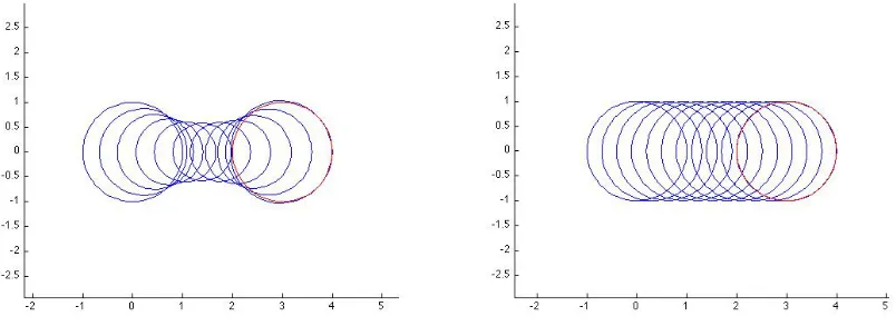
Then, the shooting algorithm can be applied, giving the diffeomorphism shown in Figure 1.
Figure 1. Constant volume experiment, left: initial (blue) and target (red), matching (right).
Figure 2. Matching trajectories without constraints (left) and with constant volume (right).
Multishape Matching. We now consider the multishape problem. In this situation, we consider shape spaces M1, M2, with M1 =M2 =C0(S1,R2) and a background space M3 =M1×M2. Elements of M3 are couples q3= (q13, q23), withq
j
3∈Mj,j = 1,2.
We take an initial stateq0= (q1, q2, q3) satisfying q31=q1, andq23=q2.
To each j ∈ {1,2,3} is associated a Hilbert space Vj of vector fields, with total control space the Hilbert
spaceV1×V2×V3.
We will consider two types of compatibility constraints between homologous curvesqj and q3j, namely
(1) Identity (or stitched) constraint: qj =q j 3
(2) Identity up to reparametrization (or sliding) constraint: q3j =qj◦f for some (time-dependent)
diffeo-morphism ofS1.
Note that, since the curves have the same initial condition, the last constraint is equivalent to assuming that ˙
qj3−q˙j◦f is tangent toq3j, i.e., taking controls (v1, v2, v3),
(v3(t, q j
for allt, where ν3j is the normal vector toq3j.
For the numerical computations, the curves are discretized into polygonal lines, and the discretization of control equations and objective functions are done by reduction to landmarks space. The discretization of the constraint in the identity case is straightforward. For each j = 1,2 and each line segment `= [z`−, z`+] in q3,j
(represented as a polygonal line), we simply use the constraint
ν`·(vj(`)−v3(`)) = 0
whereν`is the unit normal to `(unit vector perpendicular ofz`+−z−`) and
vj(`) =
1 2(vj(z
−
` ) +vj(z`+)).
Note that the verticesz`− andz+` are already part of the state variables that are obtained after discretizing the background boundariesq3.
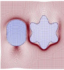
Given these choices, we can apply a minimization algorithm. In Figure 3, we provide an example comparing the two constraints. The desired transformation, as depicted in Figure 3, moves a curve with elliptical shape upward, and a flower-shaped curve downward, each curve being subject to a small deformation. The solutions obtained using the stitched and sliding constraints are provided in Figure 4, in which we have also drawn a deformed grid, representing the diffeomorphisms induced by the vector fields v1, v2 and v3 in their relevant
regions.
Figure 3. Multishape Experiment: Initial (blue) and target (red) sets of curves.
References
[1] S. Arguill`ere, E. Tr´elat, A. Trouv´e, L. Youn`es,Shape deformation analysis from the optimal control viewpoints, preprint (2013). [2] V. Arnold,Sur la g´eom´etrie diff´erentielle des groupes de Lie de dimension infinie et ses applications `a l’hydrodynamique des
fluides parfaits, Ann. Inst. Fourier16(1966), fasc. 1, 319–361.
[3] V. Arnold,Mathematical methods of classical mechanics, Graduate Texts in Mathematics60, Springer-Verlag, New York, 1989.
[4] B. Avants, J.C. Gee,Geodesic estimation for large deformation anatomical shape averaging and interpolation, Neuroimage 23(2004), S139–S150.
[5] M.F. Beg, M.I. Miller, A. Trouv´e, L. Youn`es,Computing large deformation metric mappings via geodesic flows of diffeomor-phisms, Int. J. Comput. Vis.61(2005), no. 2, 139–157.
Figure 4. Multishape Experiment, stitched (left) and sliding (right) constraints.
[7] R.F. Hartl, S.P. Sethi, R.G. Vickson,A survey of the maximum principles for optimal control problems with state constraints, SIAM Rev.37(1995), no. 2, 181–218.
[8] D.D. Holm, J. Marsden, T.S. Ratiu, Euler-Poincar´e models of ideal fluids with nonlinear dispersion, Phys. Rev. Lett.80 (1998), no. 19, 4173–4176.
[9] S.C. Joshi, M.I. Miller, Landmark matching via large deformation diffeomorphisms, IEEE Transcript Image Processing 9 (2000), no. 8, 1357–1370.
[10] J.E. Marsden, T.S. Ratiu, Introduction to mechanics and symmetry, Texts in Applied Mathematics 17, second edition, Springer-Verlag, New York, 1999.
[11] M.I. Miller, A. Trouv´e, L. Youn`es, On the metrics and Euler-Lagrange equations of computational anatomy, Annu. Rev. Biomed. Eng.4(2002), 375–405.
[12] M.I. Miller, A. Trouv´e, L. Youn`es,Geodesic shooting for computational anatomy, J. Math. Imaging Vision24(2006), no. 2, 209–228.
[13] L.S. Pontryagin, V.G. Boltyanskii, R.V. Gamkrelidze, E.F. Mishchenko, The mathematical theory of optimal processes, A Pergamon Press Book, The Macmillan Co., New York, 1964.
[14] E. Tr´elat,Contrˆole optimal (French) [Optimal control], Th´eorie & applications [Theory and applications], Math. Concr`etes [Concrete Mathematics], Vuibert, Paris, 2005.
[15] A. Trouv´e,Action de groupe de dimension infinie et reconnaissance de formes, C. R. Acad. Sci. Paris S´er. I Math.321(1995), no. 8, 1031–1034.
[16] A. Trouv´e, Diffeomorphism groups and pattern matching in image analysis, International Journal of Computational Vision 37(2005), no. 1, 17 pages.
[17] A. Trouv´e, L. Youn`es,Shape spaces, in: Handbook of Mathematical Methods in Imaging, O. Scherzer ed., Springer New York, 2011, 1309–1362.