The value of satellite remote sensing soil moisture data and the DISPATCH algorithm in irrigation fields

https://doi.org/10.5194/hess-22-5889-2018 © Author(s) 2018. This work is distributed under the Creative Commons Attribution 4.0 License.

The value of satellite remote sensing soil moisture data and the

DISPATCH algorithm in irrigation fields

Mireia Fontanet1,2,3, Daniel Fernàndez-Garcia2,3, and Francesc Ferrer1

1_{LabFerrer, Cervera, 25200, Spain}

2_{Department of Civil and Environmental Engineering, Universitat Politècnica de Catalunya (UPC),}

Barcelona, 08034, Spain

3_{Associated Unit: Hydrogeology Group (UPC-CSIC)}

Correspondence:Mireia Fontanet ([email protected]) Received: 26 February 2018 – Discussion started: 5 April 2018

Revised: 6 October 2018 – Accepted: 25 October 2018 – Published: 14 November 2018

Abstract.Soil moisture measurements are needed in a large number of applications such as hydro-climate approaches, watershed water balance management and irrigation schedul-ing. Nowadays, different kinds of methodologies exist for measuring soil moisture. Direct methods based on gravimet-ric sampling or time domain reflectometry (TDR) techniques measure soil moisture in a small volume of soil at few par-ticular locations. This typically gives a poor description of the spatial distribution of soil moisture in relatively large agriculture fields. Remote sensing of soil moisture provides widespread coverage and can overcome this problem but suf-fers from other problems stemming from its low spatial res-olution. In this context, the DISaggregation based on Phys-ical And TheoretPhys-ical scale CHange (DISPATCH) algorithm has been proposed in the literature to downscale soil mois-ture satellite data from 40 to 1 km resolution by combin-ing the low-resolution Soil Moisture Ocean Salinity (SMOS) satellite soil moisture data with the high-resolution Normal-ized Difference Vegetation Index (NDVI) and land surface temperature (LST) datasets obtained from a Moderate Res-olution Imaging Spectroradiometer (MODIS) sensor. In this work, DISPATCH estimations are compared with soil mois-ture sensors and gravimetric measurements to validate the DISPATCH algorithm in an agricultural field during two dif-ferent hydrologic scenarios: wet conditions driven by rainfall events and wet conditions driven by local sprinkler irrigation. Results show that the DISPATCH algorithm provides appro-priate soil moisture estimates during general rainfall events but not when sprinkler irrigation generates occasional het-erogeneity. In order to explain these differences, we have

ex-amined the spatial variability scales of NDVI and LST data, which are the input variables involved in the downscaling process. Sample variograms show that the spatial scales as-sociated with the NDVI and LST properties are too large to represent the variations of the average soil moisture at the site, and this could be a reason why the DISPATCH algo-rithm does not work properly in this field site.

1 Introduction

Soil moisture measurements taken over different spatial and temporal scales are increasingly required in a wide range of environmental applications, which include crop yield fore-casting (Holzman et al., 2014), irrigation planning (Vellidis et al., 2016), early warnings for floods and droughts (Koriche and Rientjes, 2016), and weather forecasting (Dillon et al., 2016). This is mostly due to the fact that soil moisture con-trols the water and energy exchanges between key environ-mental compartments (atmosphere and earth) and hydrolog-ical processes, such as precipitation, evaporation, infiltration and runoff (Ochsner, 2013; Robock et al., 2000).

information for field irrigation scheduling, determining to a great extent the duration and frequency of irrigation needed for plant growth as a function of water availability (Blonquist et al., 2006; Jones, 2004; Campbell, 1982).

Soil moisture is highly variable in space and time, mainly as a result of the spatial variability in soil properties (Haw-ley, 1983), topography (Burt and Butcher, 1985), land uses (Fu and Gulinck, 1994), vegetation (Le Roux et al., 1995) and atmospheric conditions (Koster and Suarez, 2001). As a result, soil moisture data exhibits a strong scale effect that can substantially affect the reliability of predictions, depend-ing on the method of measurement used. For this reason, it is important to understand how to measure soil moisture for irrigation scheduling.

Nowadays, available techniques for measuring or estimat-ing soil moisture can provide data either at a small or at a large scale. Gravimetric measurements (Gardner, 1986) esti-mate soil moisture by the difference between the natural and the dry weight of a given soil sample. They are used as a ref-erence value of soil moisture for sensor calibration (Starr and Paltineanu, 2002) or soil moisture validation studies (Bosch et al., 2006; Cosh et al., 2006). The main disadvantage of this method is that these measurements are time-consuming; users have to go to the field to collect soil samples and place them in the oven for a long time. Soil moisture sen-sors such as time domain reflectometry sensen-sors (Clarke Topp and Reynolds, 1998; Schaap et al., 2003; Topp et al., 1980) or capacitance sensors (Bogena et al., 2007; Dean et al., 1987) are capable of measuring soil moisture continuously using a data logger, thereby enabling the final user to save time. Soil moisture sensors are especially useful for studying pro-cesses at a small scale, but suffer from the typical low num-ber of in situ sensors that provide an incomplete picture of a large area (Western et al., 1998). Nevertheless, the use of soil moisture sensors is a common practice for guiding irrigation scheduling in cropping field systems (Fares and Polyakov, 2006; Thompson et al., 2007; Vellidis et al., 2008).

Remote sensing can estimate soil moisture continuously over large areas (Jackson et al., 1996). In this case, soil moisture estimations refer to the near-surface soil mois-ture (NSSM), which represents the first 5 cm (or less) of the top soil profile. In recent years, remote sensing tech-niques have improved and diversified their estimation, mak-ing them an interestmak-ing tool for monitormak-ing NSSM and other variables such as the Normalized Difference Vegetation In-dex (NDVI) and the land surface temperature (LST). Dif-ferent satellites exist that are capable of estimating NSSM: the Soil Moisture Active Passive (SMAP) satellite, the Ad-vanced Scatterometer (ASCAT) remote sensing instrument on board the Meteorological Operational (METOP) satellite, the Advanced Microwave Scanning Radiometer 2 (AMSR2) instrument on board the Global Change Observation Mission 1-Water (GCOM-W1) satellite, and the Soil Moisture and Ocean Salinity (SMOS) satellite launched in November 2009 (Kerr et al., 2001). The SMOS satellite has global coverage

and a revisit period of 3 days at the Equator, giving two soil moisture estimations, the first one taken during the ascend-ing overpass at 06:00 LST (local solar time) and the second one during the descending overpass at 18:00 LST. The SMOS satellite is a passive 2-D interferometer operating at L-band frequency (1.4 GHz) (Kerr et al., 2010). The spatial resolu-tion ranges from 35 to 55 km, depending on the incident an-gle. Its goal is to retrieve NSSM with a target accuracy of a 0.04 m3m−3(Kerr et al., 2012). Since SMOS NSSM values have been validated on a regular basis since the beginning of its mission (Bitar et al., 2012; Delwart et al., 2008), they is considered suitable for hydro-climate applications (Lievens et al., 2015; Wanders et al., 2014).

The relatively large variability of soil moisture compared to the low resolution of SMOS-NSSM data hinders the di-rect application of this method to irrigation scheduling. How-ever, the need for estimating NSSM with a resolution higher than 35–55 km using remote sensing has increased for dif-ferent reasons: (1) data are freely available, (2) a field instal-lation of soil moisture sensors is not necessary, and (3) no specific maintenance is needed. For these reasons, in the last few years, different algorithms have been developed to down-scale remote sensing soil moisture data to tens or hundreds of meters.

Chauhan et al. (2003) developed a Polynomial fitting method which estimates soil moisture at 1 km resolution (Carlson, 2007; Wang and Qu, 2009). This method links soil moisture data with surface temperature, vegetation index and albedo. It does not require in situ measurements but cannot be used under cloud coverage conditions. The improvements in the detection method reported by Narayan et al. (2006) downscales soil moisture at 100 m resolution. This is an op-timal resolution for agricultural applications, but the method is highly dependent on the accuracy of its input data. The same problem is attributed to the Baseline algorithm for the SMAP satellite (Das and Mohanty, 2006), which downscales soil moisture at 9 km resolution. These algorithms have to be validated using in situ measurements. For this purpose, most studies use soil moisture sensors installed at the top soil pro-file, i.e., the first 5 cm of soil (Albergel et al., 2011; Cosh et al., 2004; Jackson et al., 2010), while others use gravimet-ric soil moisture measurements (Merlin et al., 2012) or the combination of both methodologies (Robock et al., 2000). Satellite soil moisture has recently been used to provide irri-gation detection signals (Lawston et al., 2017), quantify the amount of water applied (Brocca et al., 2018; Zaussinger et al., 2018) and estimate the water use (Zaussinger et al., 2018). All these deal with relatively homogeneous and ex-tensive irrigation surface coverages (several kilometers).

be used for solving a wide range of problems related to Earth surface monitoring, such as soil moisture, but it is not a direct measurement and therefore data processing is needed. In this case, the GRD product is converted into radar backscatter coefficients and then into decibels to estimate soil moisture. Usually, these conversions are cumbersome because these kind of measurements have surface roughness and vegeta-tion influence that affect the signal (Garkusha et al., 2017; Wagner et al., 2010).

The DISPATCH method (DISaggagregation based on Physical And Theoretical CHange) (Merlin et al., 2008, 2012) is an algorithm that downscales SMOS NSSM data from 40 km (low resolution) to 1 km resolution (high res-olution). This algorithm uses Terra and Aqua satellite data to estimate NDVI and LST twice a day using the Moder-ate Resolution Imaging Spectroradiometer (MODIS) sensor. These estimations have a resolution of 1 km and can be con-ducted only if there is no cloud cover. This downscaling pro-cess provides the final user with the possibility of estimating NSSM using remote sensing techniques at high resolution. DISPATCH successfully reveals spatial heterogeneities such as rivers, large irrigation areas and floods (Escorihuela and Quintana-Seguí, 2016; Malbéteau et al., 2015, 2017; Molero et al., 2016) and it has also been validated (Malbéteau et al., 2015; Merlin et al., 2012; Molero et al., 2016) in fairly large and homogeneous irrigation areas, but it has not been applied in complex settings with spatially changing hydrologic con-ditions such as those representing a local irrigation field.

In this work, we evaluate the value of remote sensing in agricultural irrigation scheduling by comparing in situ soil moisture data obtained from gravimetric and soil moisture sensors, with soil moisture data determined by downscaling remote sensing information with the DISPATCH algorithm. Study area

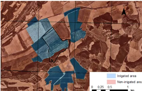
The study area shown in Fig. 1 is located in the village of Foradada (1.015◦N, 41.866◦W), in the Segarra–Garrigues (SG) system (Lleida, Catalonia). The SG system is an im-portant irrigation development project currently being car-ried out in the province of Lleida, Catalonia, which involves converting most of the current dry-land fields into irrigated fields. Its construction enables 1000 new hectares with a long agricultural tradition to be irrigated. To achieve this, an 85 km long channel was constructed to supply water for irri-gation. At present, approximately 16 000 irrigators are poten-tial beneficiaries of these installations. However, most farm-ers have not yet installed this irrigation system, which means that the SG systems can still be regarded as dry land.

The Urgell area is located in the west of the SG system. This area has totally different soil moisture conditions, es-pecially during the summer season when the majority of fields are currently irrigated. This gives rise to two clearly distinguishable wet and dry soil moisture conditions. Fig-ure 1 shows the Foradada field, which represents 25 ha of

a commercial field irrigated by a solid set sprinkler irriga-tion system distributed across 18 different irrigairriga-tion sectors. The soil texture, in a single point, is 65.6 % clay, 17.6 % silt and 16.8 % sand. Every year two different crops are grown, the first one during the winter and spring seasons, when wet conditions are maintained by precipitation, and the second one during the summer and autumn seasons, when wet con-ditions are maintained by sprinkler irrigation. The Foradada field is thus one of the few irrigated fields located within the SG system. Consequently, this field has soil moisture con-ditions similar to those in the surrounding area during the winter and spring season, but completely different conditions during the summer and autumn seasons. This makes this site unique for assessing remote sensing in a distinct isolated ir-rigation field.

2 Materials and methods

2.1 In situ soil moisture measurements

A total of nine intensive and strategic field campaigns were conducted in the study area during 2016: DOY42, DOY85, DOY102, DOY187, DOY194, DOY200, DOY215, DOY221 and DOY224. During each field campaign, disturbed soil samples were collected from the top soil profile (0–5 cm depth) for measuring gravimetric soil moisture data. A total of 101 measurement points, depicted in Fig. 1, were defined around the field. They are divided into two different kinds of points: (1) cross section points – 75 points defined to repre-sent the spatial variability of soil moisture in different cross sections (in these cross sections, points are separated by 9, 16 and 35 m); (2) support points – 26 points defined to com-plement information measured from cross sections, thereby adding and supporting information about the spatial variabil-ity across the field. Each soil sample is analyzed using the gravimetric method for measuring gravimetric soil moisture content, which is transformed to volumetric soil moisture content using bulk density measurements (Letelier, 1982). Daily averages of gravimetric measurements and their stan-dard deviations were computed to represent the soil moisture associated with the entire field site.

Figure 1. Location of the Foradada field site within the Segarra-Garriga irrigation system and distribution of soil moisture measurement points. Gravimetric measurement points are arranged with cross section points in green and support points in yellow. The location of EC-5 sensors are represented in red.

2.2 DISPATCH soil moisture measurements

In this section we briefly describe the DISPATCH algorithm. Further details can be found in Merlin et al. (2013) and refer-ences therein. The DISPATCH algorithm aims to downscale NSSM data obtained from SMOS at 40 km resolution to 1 km resolution. The method assumes that NSSM is a linear func-tion of the soil evaporative efficiency (SEE), which can be estimated at high resolution (1 km) from the acquisition of two products obtained from MODIS, i.e., LST and NDVI datasets. This MODIS-derived SEE is further considered as a proxy for the NSSM variability within the SMOS pixel. The estimation of SEE is assumed to be approximately constant during the day given clear sky conditions. The downscaling relationship is given by Eq. (1):

θHR=θSMOS+θHR0 (SEESMOS)×(SEEHR−SEESMOS) , (1)

whereθSMOSis the low-resolution SMOS soil moisture data,

SEEHR is the MODIS-derived SEE at a high resolution

(1 km), SEESMOSis the average of SEEHRwithin the SMOS

pixel at a low resolution (40 km), and θ_HR0 (SEESMOS) is

the partial derivative of soil moisture with respect to the soil evaporative efficiency at high resolution evaluated at the SEESMOS value. This partial derivative is typically

es-timated by using the linear soil evaporative efficiency model of Budyko (1956) and Manabe (1969), which is defined in Eq. (2):

θHR=SEEHR×θp, (2)

whereθHR represents the soil moisture of the top soil layer

(0–5 cm) at high resolution, andθpis an empirical parameter

that depends on soil properties and atmospheric conditions. The soil evaporation efficiency at high-resolution SEEHRis

estimated as a linear function of the soil temperature at high resolution (Ts,HR):

SEEHR=

Ts,max−Ts,HR Ts,max−Ts,min

. (3)

The soil temperature at high resolution is estimated by parti-tioning the MODIS surface temperature data (LST) into the soil and the vegetation component according to the trapezoid method of Moran et al. (1994). This also requires an estima-tion of the fracestima-tional vegetaestima-tion cover, which is calculated from the NDVI data.Ts,minandTs,maxare the soil

tempera-ture end-members (Merlin et al., 2012).

In this work, the DISPATCH algorithm has been applied during the period from DOY36 to DOY298 of 2016 to es-timate NSSM at 1 km resolution in the Foradada field site. DISPATCH provides a daily NSSM pixel map (regular grid). The Foradada field site is entirely included in one pixel. In this pixel, 51.5 % of the total area corresponds to irrigated area. The remaining portion of the pixel corresponds to dry land (shown in Fig. 2).

Figure 2.The DISPATCH grid representing the Foradada field, out-lined in dark blue, irrigated fields in light blue, and dry land in light red.

of the attributes of interest at the ground surface. This is typ-ically determined based on the type of satellite sensor. The spatial variability refers to the variations of the attributes pre-sented in the image at the ground surface, e.g., patterns of spatial continuity, size of objects in the scene, and so on. In random field theory and geostatistics, the spatial variability is mainly characterized by the covariance function or by its equivalent, the semivariogram, which is defined by (Journel and Huijbregts, 1978):

γ (h)=1 2E

n

[Z (x+h)−Z (x)]2o, (4) whereZ(x)is the random variable at thexposition, andE{·} is the expectation operator. Essentially, the semivariogram is a function that measures the variability between pairs of vari-ables separated by a distanceh. Very often, the correlation between two variables separated by a certain distance disap-pears when |h|becomes too large. At this instant,γ (h) ap-proaches a constant value. The distance beyond whichγ (h) can be considered to be a constant value is known as the range, which represents the transition of the variable to the state of negligible correlation. Thus, the range can ultimately be seen as the size of independent objects in the image. If the pixel size is smaller than 10 times the minimum range (in the absence of the nugget effect), then neighboring pixels will be alike, containing essentially the same level of information (Journel and Huijbregts, 1978). This will be a critical point in the discussion of the results later on. We note that the spatial resolution and the spatial variability are two related concepts. Several authors note that a rational choice of the spatial reso-lution for remote sensing should be based on the relationship between spatial resolution and spatial dependence (Atkinson and Curran, 1997; Curran, 1988). However, since this is not the usual procedure, the spatial resolution can be inappro-priate in some cases or provide unnecessary data in others (Atkinson and Curran, 1997; Woodcock and Strahler, 1987).

3 Results

3.1 General observations

One of the main advantages of our experiment is that remote sensing soil moisture data is evaluated during two different hydrologic periods of the same year in a given agriculture field site. The first period represents crop growth with soil wet conditions caused by natural rainfall events (without irri-gation). This period occurs during the winter and spring sea-son, i.e., from February to June. The following period occurs during the dry season with artificially created wet soil condi-tions caused by sprinkler irrigation operating to satisfy crop water requirements during the summer and autumn season, from June to October. In contrast to the rainfall events, sprin-kler irrigation creates a local artificial rainfall event using several rotating sprinkler heads. The comparisons of these two hydrologic periods allow us to evaluate the effect of lo-cal sprinkler irrigation on remote sensing soil moisture esti-mations.

Figure 3 compares gravimetric and soil moisture sensor measurements with the DISPATCH soil moisture estimates obtained from remote sensing data during the first period of time (without irrigation). We note that the comparison here is not between the point gravimetric measurements (with a support volume of few centimeters) and the satellite informa-tion (1 km in resoluinforma-tion). Instead, we compare the average of these point measurements over the entire field site (very well distributed with more than 100 measurement points) with the satellite information. The average of the soil moisture is rep-resentative of the entire irrigated area associated with the Foradada field site. Consequently, these two variables have similar support scale and are therefore comparable. Error bars in the gravimetric measurements represent the standard deviation of all the measurements obtained in 1 day. In addi-tion, the area between the light and dark green lines in this figure displays the difference between the daily minimum and maximum values of soil moisture data obtained from the five EC-5 sensors. We note that the average of the gravimet-ric soil moisture data always lies within this region. This sup-ports the use of this information to complement soil moisture data on days where no gravimetric sampling is available. The error bars associated with DISPATCH data refer to the stan-dard deviation obtained with two daily SMOS estimations and four MODIS data (two at) 06:00 LST and two more at 18:00 LST). To better appreciate tendencies, the same infor-mation is also presented as normalized relative soil moisture, i.e.,(θ−θmin)/(θmax−θmin), whereθminandθmaxare the

un-Figure 3.Comparison of average gravimetric soil moisture measurements (red) with the DISPATCH soil moisture estimations (yellow) and the daily maximum and minimum soil moisture sensor measurements (green) during the first hydrologic period (soil wet conditions caused by rainfall events only).

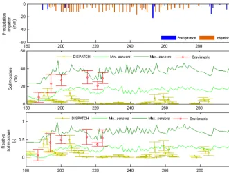
derestimates the true value of soil moisture but this could be attributed to small differences between the support volume of the field site and the spatial resolution of the satellite image. A similar analysis is shown in Fig. 4, which compares gravimetric and sensor soil moisture measurements with DISPATCH soil moisture estimations during the second pe-riod (wet soil conditions maintained by sprinkler irrigation). In contrast to our previous results, it can be seen that the DISPATCH dataset is essentially not sensitive to sprinkler irrigation even though there is a proper response to sporadic small rainfall events. Likewise, the relative increase in soil moisture measurements also shows that sprinkler irrigation does not affect the DISPATCH estimation. Thus, even though the DISPATCH estimations seem to properly respond to rain-fall events during the first period, irrigation operating at the Foradada field scale remains undetected during the second period. The DISPATCH dataset is not sensitive to irrigation and merely indicates that soil dry conditions exist at a larger scale.

This can also be seen from a different perspective by look-ing at the scatter plot between the average of the normalized relative soil moisture data obtained with the EC-5 sensors and the corresponding DISPATCH measurement determined on the same day. Figure 5 shows the scatter plots obtained during rainfall events and irrigation period. We note that even though a clear tendency is seen during rainfall events (R2=0.57), no correlation seems to exist during irrigation

(R2=0.04). We conclude then that the DISPATCH dataset provides representative estimates of soil moisture at a lower resolution than expected.

3.2 Analysis and discussion

respec-Figure 4.Comparison of average gravimetric soil moisture measurements (red) with the DISPATCH soil moisture estimations (yellow) and the daily maximum and minimum soil moisture sensor measurements (green) during the second hydrologic period (soil wet conditions caused by irrigation). The top figure shows the intensity of precipitation and irrigation.

Figure 5.Scatter plot between the average of the normalized soil moisture obtained with EC-5 sensors and the DISPATCH measurements obtained during both hydrologic scenarios, rainfall events and irrigation period.

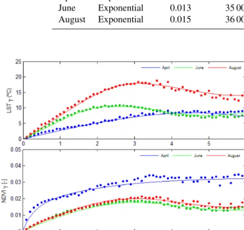
tively estimated from the MOD13A2 and MOD11A1 product data, which can be freely downloaded from the Google Earth Engine website (https://earthengine.google.com, last access: 15 January 2017). We selected daily representative images of April, June and August. The April image describes a general rainfall event in the region, the June image shows when lo-cal irrigation starts in the Foradada field, and finally the Au-gust image represents when the crop is well developed and frequent irrigation is needed. Experimental semivariograms have been fitted with a theoretical model (spherical and

expo-nential models for the LST and NDVI, respectively), which can be formally expressed as Eqs. (5) and (6):

γLST(h)=c11Sph _|h|

a11

+c12

1−cos

_|h|

a12 π

, (5)

γNDVI(h)=c21Exp _|h|

a21

+c22Exp _|h|

a22

+c23

1−cos

_|h|

a23 π

Table 1.Random function model parameters of LST semivariograms.

LST

Variogram Hole effect

Month Model Sill(c11) Range(a11) Sill(c12) Range(a12)

April Spheric 8.4 46 000 – –

June Spheric 7.5 22 000 1.5 25 000 August Spheric 14 32 000 2 29 000

Table 2.Random function model parameters of NDVI semivariograms.

NDVI

Variogram Hole effect

Month Model Sill(c21) Range(a21) Sill(c22) Range(a22) Sill(c23) Range(a23)

April Exponential 0.013 8000 0.02 55 000 – – June Exponential 0.013 35 000 – – 0.22 28 000 August Exponential 0.015 36 000 – – 0.21 28 000

Figure 6. LST and NDVI experimental and theoretical semivari-ograms associated with April (blue), June (green) and August (red).

wherecij are constant coefficients that represent the contri-bution of the different standard semivariogram models, and aij denotes the corresponding ranges of the different struc-tures. The LST and NDVI experimental and theoretical semi-variograms are shown in Fig. 6. The parameters adopted in the random function model are summarized in Tables 1 and 2. The analysis determines a nested structure with a posi-tive linear combination between isotropic stationary semivar-iogram models and the hole effect model. Hole effect struc-tures most often indicate a form of periodicity (Pyrcz and Deutsch, 2003). In our case, this periodicity reflects the pres-ence of areas with different watering and crop growth

con-ditions, i.e., in contrast to the dry-land conditions in the SG area, the Urgell area is based on irrigation.

The spatial variability of NDVI and LST vary with time according to changes in hydrologic conditions. In April, the semivariogram of NDVI displays more variability and less spatial continuity due to the differences in growth rate and crop type conditions existing at the regional scale during the wet season (controlled by rainfall events). On the other hand, the spatial dependence of LST is more significant in Au-gust. Importantly, results show that the scale of variability (range) associated with MODIS data during the dry season, when a controlled amount of water by irrigation is applied, ranges between 35 and 36 km for the NDVI and between 22 and 32 km for the LST. Recalling the discussion provided in Sect. 2.3., this means that the size of independent objects in the NDVI and LST images is about 30 km and that insignifi-cant spatial variations of NDVI and LST values are expected below 1/10 of this size. This suggests that the NDVI and LST products provided by MODIS cannot detect differences between neighboring pixels with a size of 1 km.

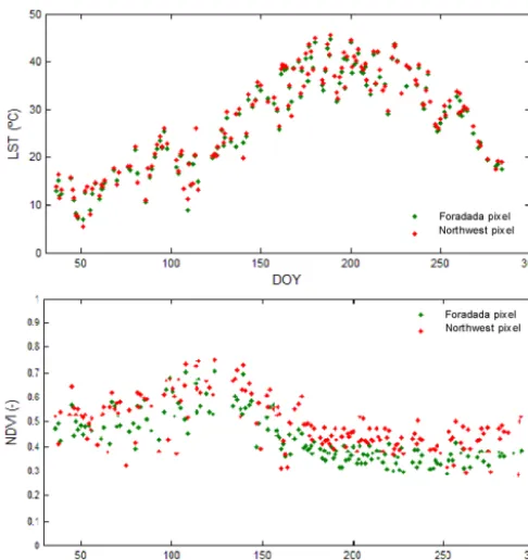
Figure 7. Temporal evolution of LST and NDVI obtained at the Foradada pixel and its neighboring northwest pixel situated 2 km away.

both pixels even when irrigation is applied. Results show that the LST and NDVI information can detect neither the sprin-kler irrigation nor the crop growth as a consequence of irri-gation in this case. We finally note that these results suggest that the resolution of LST and NDVI is not appropriate in this case but can also express that these two variables are simply not sensitive to irrigation because they only provide infor-mation about the status of the crop and land surface. Further research is needed in this sense.

4 Conclusions

We analyze the value of remote sensing and the DISPATCH downscaling algorithm for predicting soil moisture variations in an irrigated field site of size close to image resolution. The DISPATCH algorithm based on the NDVI and LST data ob-tained from the MODIS satellite is used for downscaling the SMOS information and transforming the SMOS soil mois-ture estimations from a resolution of 40 to 1 km. These esti-mates are then compared with average gravimetric and soil moisture sensor measurements taken all over the field site. Results have shown that in this case the downscaled soil moisture estimations are capable of predicting the variations in soil moisture caused by rainfall events but fail to reproduce the temporal fluctuations in the average water content caused by local irrigation. To provide insight into this problem, we examine the spatial variability of the different input variables

involved, i.e., the NDVI and LST. Results indicated that the size of individual objects in the NDVI and LST images is too large to be able to adequately represent the variations of the average water content at the site. This effect is not signifi-cant during rainfall events because the typical spatial scale of rainfall events is much larger than the size of the irrigated field site.

From a different perspective, these results also suggest that irrigation scheduling based on satellite information coupled with the DISPATCH downscaling algorithm might be appro-priate in regions of the world with extensive irrigation sur-face coverage, larger than approximately 10 km (e.g., Pun-jab basin). However, care should be taken when directly ap-plying this method as its performance will strongly depend on the spatiotemporal variation of irrigation within the area. These variations can generate occasional areas with different hydrologic scenarios and behaviors leading to the failure of the soil moisture prediction method.

Data availability. All data are available form the corresponding au-thor upon request.

Author contributions. MF, DFG and FF contributed to design and implementation of the research, to the analysis of the results and to the writing of the paper.

Competing interests. The authors declare that they have no conflict of interest.

Acknowledgements. We thank our colleagues from “Root zone soil moisture Estimates at the daily and agricultural parcel scales for Crop irrigation management and water use impact” (REC project), who provided insight and expertise that greatly assisted the research.

Edited by: Micha Werner

Reviewed by: two anonymous referees

References

Albergel, C., Zakharova, E., Calvet, J.-C., Zribi, M., Pardé, M., Wigneron, J.-P., Novello, N., Kerr, Y., Mialon A., and Fritz, N.: A first assessment of the SMOS data in southwestern France us-ing in situ and airborne soil moisture estimates: the CAROLS airborne campaign, Remote Sens. Environ., 115, 2718–2728, https://doi.org/10.1016/j.rse.2011.06.012, 2011.

Atkinson, P. and Curran, P.: Choosing an appropriate spatial reso-lution for remote sensing investigations, Photogramm. Eng. Re-mote Sens., 63, 1345–1351, 1997.

Bauer-Marschallinger, B., Freeman, V., Cao, S., Paulik, C., Schaufler, S., Stachl, T., Modanesi, S., Massari, C., Cia-batta, L., Brocca, L., and Wagner, W.: Toward Global Soil Moisture Monitoring With Sentinel-1: Harnessing Assets and Overcoming Obstacles, IEEE T. Geosci. Remote, 20, 1–20, https://doi.org/10.1109/TGRS.2018.2858004, 2018.

Blonquist, J. M., Jones, S. B., and Robinson, D. A.: Precise irri-gation scheduling for turfgrass using a subsurface electromag-netic soil moisture sensor, Agr. Water Manage., 84, 153–165, https://doi.org/10.1016/j.agwat.2006.01.014, 2006.

Bogena, H. R., Huisman, J. A., Oberdörster, C., and Vereecken, H.: Evaluation of a low-cost soil water content sensor for wireless network applications, J. Hydrol., 344, 32–42, https://doi.org/10.1016/j.jhydrol.2007.06.032, 2007.

Bosch, D. D., Lakshmi, V., Jackson, T. J., Choi, M., and Jacobs, J. M.: Large scale measurements of soil mois-ture for validation of remotely sensed data: Georgia soil moisture experiment of 2003, J. Hydrol., 323, 120–137, https://doi.org/10.1016/j.jhydrol.2005.08.024, 2006.

Brocca, L., Tarpanelli, A., Filippucci, P., Dorigo, W., Zaussinger, F., Gruber, A., and Fernández-prieto, D.: Int J Appl Earth Obs Geoinformation How much water is used for irriga-tion? A new approach exploiting coarse resolution satellite soil moisture products, Int. J. Appl. Earth Obs., 73, 752–766, https://doi.org/10.1016/j.jag.2018.08.023, 2018.

Budyko, M. I.: Heat balance from the Aquarius/SAC-D satellite: description and initial assessment, IEEE Geosci. Remote Sens. Lett., 12, 923–927, 1956.

Burt, T. P. and Butcher, D. P.: Topographic controls of soil moisture distributions, J. Soil Sci., 36, 469–486, https://doi.org/10.1111/j.1365-2389.1985.tb00351.x, 1985. Campbell, C. S. and Devices, D.: Calibrating ECH₂O Soil

Mois-ture Probes, available at: http://citeseerx.ist.psu.edu/viewdoc/ download?doi=10.1.1.559.4409&rep=rep1&type=pdf (last ac-cess: 15 February 2017), 2–4, 1986.

Campbell, G.: Soil water potential neasurements: an overview, Aca-demic Press, New York, 1982.

Carlson, T.: An overview of the “triangle method” for estimating surface evapotranspiration and soil moisture from satellite im-agery, Sensors, 7, 1612–1629, https://doi.org/10.3390/s7081612, 2007.

Chauhan, N. S., Miller, S., and Ardanuy, P.: Spaceborne soil moisture estimation at high resolution: A microwave-optical/IR synergistic approach, Int. J. Remote Sens., 24, 4599–4622, https://doi.org/10.1080/0143116031000156837, 2003.

Clarke Topp, G. and Reynolds, W. D.: Time domain reflectom-etry: A seminal technique for measuring mass and energy in soil, Soil Till. Res., 47, 125–132, https://doi.org/10.1016/S0167-1987(98)00083-X, 1998.

Clothier, B. E. and Green, S. R.: Rootzone processes and the ef-ficient use of irrigation water, Agr. Water Manag., 25, 1–12, https://doi.org/10.1016/0378-3774(94)90048-5, 1994.

Cosh, M. H., Jackson, T. J., Bindlish, R., and Prueger, J. H.: Water-shed scale temporal and spatial stability of soil moisture and its role in validating satellite estimates, Remote Sens. Environ., 92, 427–435, https://doi.org/10.1016/j.rse.2004.02.016, 2004.

Cosh, M. H., Jackson, T. J., Starks, P., and Heathman, G.: Temporal stability of surface soil moisture in the Little Washita River watershed and its applications in satellite soil moisture product validation, J. Hydrol., 323, 168–177, https://doi.org/10.1016/j.jhydrol.2005.08.020, 2006.

Curran, P. J.: The semivariogram in remote sensing: An introduction, Remote Sens. Environ., 24, 493–507, https://doi.org/10.1016/0034-4257(88)90021-1, 1988.

Das, N. N. and Mohanty, B. P.: Root Zone Soil Moisture Assess-ment Using Remote Sensing and Vadose Zone Modeling, Va-dose Zone J., 5, 296–307, https://doi.org/10.2136/vzj2005.0033, 2006.

Dean, T. J., Bell, J. P., and Baty, A. J. B.: Soil moisture measurement by an improved capacitance technique, Part I. Sensor design and performance, J. Hydrol., 93, 67–78, https://doi.org/10.1016/0022-1694(87)90194-6, 1987.

Delwart, S., Bouzinac, C., Wursteisen, P., Berger, M., Drinkwater, M., Martín-Neira, M., and Kerr, Y. H.: SMOS validation and the COSMOS campaigns, IEEE T. Geosci. Remote, 46, 695–703, https://doi.org/10.1109/TGRS.2007.914811, 2008.

Dillon, M. E., Collini, E. A., and Ferreira, L. J.: Sensi-tivity of WRF short-term forecasts to different soil mois-ture initializations from the GLDAS database over South America in March 2009, Atmos. Res., 167, 196–207, https://doi.org/10.1016/j.atmosres.2015.07.022, 2016.

Escorihuela, M. J. and Quintana-Seguí, P.: Comparison of re-mote sensing and simulated soil moisture datasets in Mediter-ranean landscapes, Remote Sens. Environ., 180, 99–114, https://doi.org/10.1016/j.rse.2016.02.046, 2016.

Fares, A. and Polyakov, V.: Advances in Crop Water Manage-ment Using Capacitive Water Sensors, Adv. Agron., 90, 43–77, https://doi.org/10.1016/S0065-2113(06)90002-9, 2006. Fu, B. and Gulinck, H.: Land evaluations in an area of severe

ero-sion: the loess plateau of China, L. Degrad. Rehabil. l. Degrad. Rehabil., 5, 33–40, 1994.

Gardner, W. H.: Water content, in: Methods of Soil Analyses, edited by: Klute, A., Agronomy Monograph 9, ASA, Madison, WI, 493–541, 1986.

Garkusha, I. N., Hnatushenko, V. V., and Vasyliev, V. V.: Us-ing Sentinel-1 data for monitorUs-ing of soil moisture, 2017 IEEE Int. Geosci. Remote Sens. Symp., 41, 1656–1659, https://doi.org/10.1109/IGARSS.2017.8127291, 2017.

Hawley, M. E.: J. Hydrol., 62, 179–200, https://doi.org/10.1016/0022-1694(83)90102-6, 1983.

Holzman, M. E., Rivas, R., and Piccolo, M. C.: International Jour-nal of Applied Earth Observation and Geoinformation Estimat-ing soil moisture and the relationship with crop yield usEstimat-ing sur-face temperature and vegetation index, Int. J. Appl. Earth Obs., 28, 181–192, 2014.

Hornacek, M., Wagner, W., Sabel, D., Truong, H.-L., Snoeij, P., Hahmann, T., Diedrich, E., and Doubkova, M.: Potential for High Resolution Systematic Global Surface Soil Moisture Retrieval via Change Detection Using Sentinel-1, IEEE J. Sel. Top. Appl., 5, 1303–1311, https://doi.org/10.1109/JSTARS.2012.2190136, 2012.

Jackson, T. J., Schugge, J., and Engman, E. T.: Remote sensing ap-plications to hydrology: soil moisture, Hydrolog. Sci. J., 41, 517– 530, https://doi.org/10.1080/02626669609491523, 1996. Jackson, T. J., Cosh, M. H., Bindlish, R., Starks, P. J., Bosch,

D. D., Seyfried, M., Goodrich, D. C., Moran, M. S., and Du, J.: Validation of advanced microwave scanning radiometer soil moisture products, IEEE T. Geosci. Remote, 48, 4256–4272, https://doi.org/10.1109/TGRS.2010.2051035, 2010.

Jones, H. G.: Irrigation scheduling: Advantages and pit-falls of plant-based methods, J. Exp. Bot., 55, 2427–2436, https://doi.org/10.1093/jxb/erh213, 2004.

Journel, A. and Huijbregts, C.: Mining geostatistics: London, Aca-demic Press, 600 pp., 1978.

Kerr, Y. H., Waldteufel, P., Wigneron, J. P., Martinuzzi, J. M., Font, J., and Berger, M.: Soil moisture retrieval from space: The Soil Moisture and Ocean Salinity (SMOS) mission, IEEE T. Geosci. Remote, 39, 1729–1735, https://doi.org/10.1109/36.942551, 2001.

Kerr, Y. H., Waldteufel, P., Wigneron, J., Delwart, S., Cabot, F., Font, J., Reul, N., Boutin, J., Gruhier, C., Juglea, S. E., Drinkwa-ter, M. R., Mecklenburg, S., Hahne, A., and Martı, M.: The SMOS Mission?: New Tool for Monitoring Key Elements of the Global Water Cycle, P. IEE, 98, 666–687, 2010.

Kerr, Y. H., Waldteufel, P., Richaume, P., Wigneron, J. P., Ferraz-zoli, P., Mahmoodi, A., Bitar, A. Al, Cabot, F., Gruhier, C., Ju-glea, S. E., Leroux, D., Mialon, A., and Delwart, S.: The SMOS Soil Moisture Retrieval Algorithm, Geosci. Remote Sens., 50, 1384–1403, https://doi.org/10.1109/TGRS.2012.2184548, 2012. Koriche, S. A. and Rientjes, T. H. M.: Application of satellite products and hydrological modelling for flood early warning, Phys. Chem. Earth, 93, 12–23, https://doi.org/10.1016/j.pce.2016.03.007, 2016.

Koster, R. D. and Suarez, M. J.: Soil Mois-ture Memory in Climate Models, J. Hydrome-teorol., 2, 558–570, https://doi.org/10.1175/1525-7541(2001)002<0558:SMMICM>2.0.CO;2, 2001.

Lawston, P. M., Santanello Jr., J. A., and V. Kumar, S.: Irrigation Signals Detected From SMAP Soil Mois-ture Retrievals, Geophys. Res. Lett., 44, 11860–11867, https://doi.org/10.1002/2017GL075733, 2017.

Le Roux, X., Bariac, T., and Mariotti, a: Spatial partitioning of the soil water resoucre between grasses and shrub compnents in a west African humid savanna, Oecologia, 104, 145–155, https://doi.org/10.1007/BF00328579, 1995.

Letelier, E.: Medición de la densidad aparente del suelo por medio de la capilaridad, Agr. Tec., 42, 77–78, 1982.

Lievens, H., Tomer, S. K., Al Bitar, A., De Lannoy, G. J. M., Dr-usch, M., Dumedah, G., Hendricks Franssen, H. J., Kerr, Y. H., Martens, B., Pan, M., Roundy, J. K., Vereecken, H., Walker, J. P., Wood, E. F., Verhoest, N. E. C., and Pauwels, V. R. N.: SMOS soil moisture assimilation for improved hydrologic simulation in the Murray Darling Basin, Australia, Remote Sens. Environ., 168, 146–162, https://doi.org/10.1016/j.rse.2015.06.025, 2015. Malbéteau, Y., Merlin, O., Molero, B., Rüdiger, C., and

Ba-con, S.: DisPATCh as a tool to evaluate coarse-scale re-motely sensed soil moisture using localized in situ measure-ments: Application to SMOS and AMSR-E data in South-eastern Australia, Int. J. Appl. Earth Obs., 45, 221–234, https://doi.org/10.1016/j.jag.2015.10.002, 2015.

Malbéteau, Y., Merlin, O., Balsamo, G., Er-Raki, S., Khabba, S., Walker, J. P., and Jarlan, L.: Towards a surface soil mois-ture product at high spatio-temporal resolution: temporally-interpolated spatially-disaggregated SMOS data, J. Hydrome-teorol., 19, 183–200, https://doi.org/10.1175/JHM-D-16-0280.1, 2017.

Manabe, S.: Climate and the ocean circulation. The atmospheric cir-culation and the hydrology of the Earth’s surface, Mon. Weather Rev., 97, 739–774, 1969.

Mattia, F., Satalino, G., Balenzano, A., Rinaldi, M., Steduto, P. and Moreno, J.: SENTINEL-1 FOR WHEAT MAPPING AND SOIL MOISTURE RETRIEVAL, IGARSS, 2, 2832–2835, 2015. Merlin, O., Chehbouni, G., Walker, J. P., Panciera, R., Kerr, Y.

H., Merlin, O., Chehbouni, G., Walker, J. P., Panciera, R., and Kerr, Y. H. A.: A simple methods for downscaling passive mi-crowave based soil moisture Passive mimi-crowave soil moisture downscaling using evaporative fraction Olivier Merlin Abdel-ghani Chehbouni Jeffrey P. Walker Rocco Panciera Yann Kerr Centre d’Etudes Spatiales de la, IEEE Geosci. Remote S., 46, 786–769, 2008.

Merlin, O., Jacob, F., Wigneron, J. P., Walker, J., and Chehbouni, G.: Multidimensional disaggregation of land surface temperature using high-resolution red, near-infrared, shortwave-infrared, and microwave-L bands, IEEE T. Geosci. Remote, 50, 1864–1880, https://doi.org/10.1109/TGRS.2011.2169802, 2012.

Merlin, O.: An original interpretation of the wet edge of the sur-face temperature-albedo space to estimate crop evapotranspi-ration (SEB-1S), and its validation over an irrigated area in northwestern Mexico, Hydrol. Earth Syst. Sci., 17, 3623–3637, https://doi.org/10.5194/hess-17-3623-2013, 2013.

Molero, B., Merlin, O., Malbéteau, Y., Al Bitar, A., Cabot, F., Stefan, V., Kerr, Y., Bacon, S., Cosh, M. H., Bindlish, R., and Jackson, T. J.: SMOS disaggregated soil mois-ture product at 1 km resolution: Processor overview and first validation results, Remote Sens. Environ., 180, 361–376, https://doi.org/10.1016/j.rse.2016.02.045, 2016.

Moran, M. S., Clarke, T. R., Inoue, Y., and Vidal, A.: Esti-mating crop water defficiency using the relation between sur-face minus air temperature and spectral vegetation index, Re-mote Sens. Environ., 49, 246–263, https://doi.org/10.1016/0034-4257(94)90020-5, 1994.

Narayan, U., Lakshmi, V., and Jackson, T. J.: High resolution esti-mation of soil moisture using L-band radiometer and radar obser-vations made during trhe SMEX02 experiments, IEEE T. Geosci. Remote, 44, 1545–1554, 2006.

Oschsner, T. E., Cosh, M. H., Cuenca, R. H., Dorigo, W. A., Draper, C. S., Hagimoto, Y., and Zreda, M.: State of the art in large-scale soil moisture monitoring, Soil Sci. Soc. Am. J., 77, 1888–1919, https://doi.org/10.2136/sssaj2013.03.0093, 2013.

Paloscia, S., Pettinato, S., Santi, E., Notarnicola, C., Pasolli, L., and Reppucci, A.: Soil moisture mapping using Sentinel-1 images: Algorithm and preliminary validation, Remote Sens. Environ., 134, 234–248, https://doi.org/10.1016/j.rse.2013.02.027, 2013. Pyrcz, M. and Deutsch, C.: The whole story on the hole effect,

Geo-statistical Assoc. Australas. Newsl., 18, 3–5, 2003.

Me-teorol. Soc., 81, 1281–1299, https://doi.org/10.1175/1520-0477(2000)081<1281:TGSMDB>2.3.CO;2, 2000.

Schaap, M. G., Robinson, D. a., Friedman, S. P., and Lazar, a.: Measurement and Modeling of the TDR Signal Propagation through Layered Dielectric Media, Soil Sci. Soc. Am. J., 67, 1113, https://doi.org/10.2136/sssaj2003.1113, 2003.

Starr, J. L. and Paltineanu, I. C.: Methods for Measurement of Soil Water Content: Capacitance Devices, in: Dane, J. H. and Topp, G. C., Methods of Soil Analysis: Part 4 Physical Methods, Soil Science Society of America, Inc., Soil Science Society of Amer-ica, Inc., 463–474, 2002.

Thompson, R. B., Gallardo, M., Valdez, L. C., and Fernán-dez, M. D.: Using plant water status to define threshold values for irrigation management of vegetable crops using soil moisture sensors, Agr. Water Manage., 88, 147–158, https://doi.org/10.1016/j.agwat.2006.10.007, 2007.

Topp, G. C., Davis, J. L., and Annan, A. P.: Electromagnetic Determination of Soil Water Content: Measruements in Coax-ial Transmission Lines, Water Resour. Res., 16, 574–582, https://doi.org/10.1029/WR016i003p00574, 1980.

Vellidis, G., Tucker, M., Perry, C., Kvien, C., and Bed-narz, C.: A real-time wireless smart sensor array for scheduling irrigation, Comput. Electron. Agr., 61, 44–50, https://doi.org/10.1016/j.compag.2007.05.009, 2008.

Vellidis, G., Liakos, V., Perry, C., Porter, W. M., and Tucker, M. A.: Irrigation Scheduling for Cotton Using Soil Moisture Sen-sors, Smartphone Apps, and Traditional Methods, National Cot-ton Council, Memphis, TN, paper 16779, 772–780, 2016.

Wagner, W., Sabel, D., Doubkova, M., Bartsch, A., and Pathe, C.: The Potential of Sentinel-1 for Monitoring Soil Moisture with a high Spatial Resolution at Global Scale, ESA Spec. Publ. SP-674, 5, 2010.

Wanders, N., Karssenberg, D., de Roo, A., de Jong, S. M., and Bierkens, M. F. P.: The suitability of remotely sensed soil mois-ture for improving operational flood forecasting, Hydrol. Earth Syst. Sci., 18, 2343–2357, https://doi.org/10.5194/hess-18-2343-2014, 2014.

Wang, L. and Qu, J. J.: Satellite remote sensing applications for sur-face soil moisture monitoring: A review, Front. Earth Sci. China, 3, 237–247, https://doi.org/10.1007/s11707-009-0023-7, 2009. Western, A. W., Blöschl, G., and Grayson, R. B.: Geostatistical

characterisation of soil moisture patterns in the Tarrawarra catch-ment, J. Hydrol., 205, 20–37, https://doi.org/10.1016/S0022-1694(97)00142-X, 1998.

Woodcock, C. E., and Strahler, A. H.: the Factor of Scale in Remote-Sensing, Remote Sens. Environ., 21, 311–332, https://doi.org/10.1016/0034-4257(87)90015-0, 1987.