Applied Probabilistic
Forecasting
Author:
Roman
Binter
London, December 17, 2012
I certify that the thesis I have presented for examination for the MPhil/PhD degree of the London School of Economics and Political Science is solely my own work other than where I have clearly indicated that it is the work of others (in which case the extent of any work carried out jointly by me and any other person is clearly identified in it).
The copyright of this thesis rests with the author. Quotation from it is permitted, provided that full acknowledgement is made. This thesis may not be reproduced without my prior written consent.
I warrant that this authorisation does not, to the best of my belief, infringe the rights of any third party.
In any actual forecast, the future evolution of the system is uncertain and the forecasting model is mathematically imperfect. Both, ontic uncertainties in the future (due to true stochasticity) and epistemic uncertainty of the model (reflecting structural imperfections) complicate the construction and evalu-ation of probabilistic forecast. In almost all nonlinear forecast models, the evolution of uncertainty in time is not tractable analytically and Monte Carlo approaches (”ensemble forecasting”) are widely used. This thesis advances our understanding of the construction of forecast densities from ensembles, the evolution of the resulting probability forecasts and methods of establish-ing skill (benchmarks). A novel method of partially correctestablish-ing the model error is introduced and shown to outperform a competitive approach.
The properties of Kernel dressing, a method of transforming ensembles into probability density functions, are investigated and the convergence of the approach is illustrated. A connection between forecasting and Information theory is examined by demonstrating that Kernel dressing via minimization of Ignorance implicitly leads to minimization of Kulback-Leibler divergence. The Ignorance score is critically examined in the context of other Information theory measures.
of global circulation models of the ENSEMBLES project. ENSEMBLES is a project funded by the European Union bringing together all major European weather forecasting institutions in order to develop and test state-of-the-art seasonal weather forecasting models. Via benchmarking the seasonal fore-casts of the ENSEMBLES models we demonstrate that Dynamic Climatology can help us better understand the value and forecasting performance of large scale circulation models.
I would like to thank my supervisor Prof. Leonard A. Smith for his relentless support that he so generously provided me with throughout the development of this thesis. My very special thanks goes to him for offering me the ‘blue pill’1 and giving me the opportunity to peak into the world behind the mirror.
I would also like to thank all the past and present crew of the Centre for the Analysis of Time Series for being wonderful CATS, as well as members of the Department of Statistics for being inspirational friends, colleagues and teachers.
1 Introduction 34
2 Background 42
2.1 Forecasting . . . 43
2.1.1 System model pair . . . 45
2.1.2 Forecasting framework . . . 46
2.1.3 Perfect and imperfect model scenario . . . 48
2.1.4 Sources of uncertainty in physical systems . . . 50
2.2 Probabilistic forecasting . . . 52
2.2.1 Ensemble forecasting and forecasting densities . . . 52
2.2.2 Constructing forecasting densities . . . 54
2.2.3 Unconditional climatology and climatological forecast . 57 2.2.4 Conditional climatology . . . 58
2.2.5 Blending climatological and model forecasts . . . 59
2.3.1 Information-based measures of performance . . . 63
2.3.2 Forecast performance and optimal compression . . . 64
2.4 Probabilistic forecast evaluation . . . 65
2.4.1 Background on forecast evaluation . . . 66
2.4.2 Ignorance and other scoring rules . . . 67
2.4.3 Kernel dressing . . . 71
2.4.4 Crossvalidation and subsampling . . . 74
2.5 Seasonal forecasting . . . 75
2.5.1 Seasonal forecasting and models . . . 75
2.5.2 Long-term patterns and regions of importance . . . 76
2.5.3 The ENSEMBLES models . . . 78
2.5.4 Multi-model ensembles in seasonal forecasting . . . 79
2.5.5 Benchmark models and their value . . . 81
2.6 Correcting a model error . . . 82
2.6.1 Systematic part of a model error . . . 83
2.6.2 Iterative vs. direct predictors . . . 84
2.6.3 Correction models . . . 84
2.6.4 Applications and limitations of correction models . . . 86
3.1.1 Perfect model testbed . . . 90
3.1.2 Distinguishing Kernel dressing and Kernel density Es-timation . . . 92
3.1.3 Ignorance as a minimizer of Kullback-Leibler divergence 94 3.2 Numerical analysis of Kernel Dressing properties . . . 96
3.2.1 Convergence in perfect model scenario . . . 97
3.2.2 Archive size and archive-ensemble size tradeoff . . . 104
3.2.3 Kernel Dressing outside perfect model scenario . . . 108
3.2.4 Affine kernel dressing outside perfect model scenario . 111 3.3 Linking information measures . . . 114
3.3.1 Roulette, a punter, and the house . . . 114
3.3.2 Forecasting the roulette outcome . . . 115
3.3.3 Growth of punter’s wealth . . . 117
3.3.4 Scenario: Punter, the house both know true probabilities119 3.3.5 Scenario: Only the house knows the true probabilities . 120 3.3.6 Scenario: None knows the true probabilities . . . 121
3.4 Conclusions . . . 122
4 Dynamic climatology and its benchmarking utility 126 4.1 Dynamic climatology . . . 130
4.1.1 Analogs, and how to find them . . . 130
4.1.3 Growing ensembles . . . 135
4.1.4 Pruning the ensembles . . . 136
4.1.5 The DC parameters, further comments . . . 137
4.2 Numerical illustration . . . 138
4.2.1 Demonstration using a sine function . . . 139
4.2.2 Demonstration using forced damped pendulum . . . 143
4.3 Application: DC Benchmarking of ENSEMBLES . . . 151
4.3.1 Experimental design issues and DC calibration . . . 152
4.3.2 ENSEMBLES, DC performance in Nino 3.4 . . . 155
4.3.3 ENSEMBLES, DC performance in MDR . . . 163
4.4 Conclusions . . . 168
5 Forecasting with Radial Basis Functions 171 5.1 Model fit and ensemble forecast . . . 172
5.1.1 Interpolating with Radial Basis Functions . . . 172
5.1.2 Interpolation, approximation, and computational cost . 177 5.1.3 Training for forecasting . . . 179
5.1.4 Generating an ensemble forecast . . . 180
5.2 Center selection . . . 181
5.2.1 Simple attractor covering . . . 181
5.2.3 Knot insertion . . . 184
5.2.4 Adaptive knot insertion . . . 186
5.2.5 The power function . . . 186
5.2.6 Which method to use? . . . 188
5.3 Conclusions . . . 189
6 Forecast correction: Predictor Corrector and ΨΦ 192 6.1 Constructing the core model Φ . . . 194
6.1.1 Systematic model error . . . 195
6.1.2 Generating core model ensemble forecasts . . . 196
6.1.3 Using the core model . . . 198
6.2 The ΨΦ method . . . 199
6.2.1 The core model forecast and forecasting errors . . . 199
6.2.2 Fitting the corrector, quality of the error surface . . . . 201
6.2.3 ΨΦ in forecasting mode . . . 202
6.3 The Predictor Corrector method . . . 203
6.3.1 Constructing the C-corrector . . . 204
6.3.2 Selecting center for the C-corrector . . . 206
6.3.3 Forecasting mode . . . 208
6.4 Forecasting Lorenz84/63 . . . 211
6.4.2 Limitations of RMS evaluation . . . 219
6.4.3 Impact of number of centers . . . 223
6.4.4 Dataset size and number of centers tradeoff . . . 226
6.5 Why does PC outperform ΨΦ? . . . 228
6.6 Conclusions . . . 230
A Dynamical systems 234 A.1 The Lorenz84 system . . . 234
A.2 The Lorenz63 system . . . 235
A.3 The damped forced pendulum . . . 235
B Dynamic Climatology: data and evaluation 238 B.1 Evaluation . . . 238
B.2 Pendulum dataset . . . 239
B.3 Nino34 and MDR datasets . . . 239
B.4 Probability plumes: ECMWF and Dynamic Climatology . . . 240
C The ΨΦ/PC: data, core model, and evaluation 244 C.1 The datasets . . . 244
C.2 Forecasting settings . . . 246
C.3 Data transformation . . . 247
C.5 Model specification . . . 250
C.5.1 Constructing Ψ . . . 251
C.6 Out-of-sample evaluation . . . 252
D Computational considerations of RBF and ΨΦ/PC 253
D.1 The cost RBF interpolation . . . 254
2.1 Ensemble forecast: Using an observation (large red circle) at time t = 0, an ensemble of initial conditions (small red circles at
t = 0) is constructed and iterated forward using the model (blue lines) to obtain an ensemble forecast (small red circles at t = 1). At time t = 1 the forecast can be verified with an outcome (red cross), i.e. system state observed at timet+ 1. . . 53
2.2 Climatological ignorance in Nino34: Forecasting performance of climatology of monthly SST temperatures over Nino3.4 region
evaluated in terms of Ignorance. Ignorance is calculated for a
vary-ing size of a phase angle (window). For window size of 6 the
condi-tional climatology becomes uncondicondi-tional, as all observations will
fall within the window. The optimal window in this case is 0 (the
lowest level of Ignorance), i.e. the climatology should condition
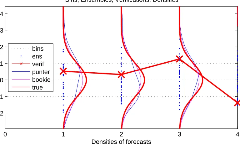
2.3 Forecast distributions (Gaussian-like curves) somewhat re-semble the true p (red Gaussian-like curve). The punter uses the (blue) ensemble members to construct her estimate (blue
Gaussian-like curve) of the truep. The bookie constructs his estimate (ma-genta) using climatological approach with all realized verifications
(red crosses joined with red line) being included in his ensembles. . 73
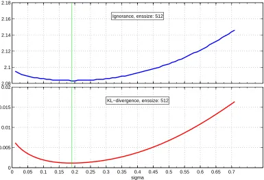
3.1 Ignorance minimizes KL-divergence (PMS): Ignorance as a func-tion of the parameter σ (top) calculated for a particular sample for a model with 512 ensemble members. The minimum value of Ignorance
(green line) coincides with the minimum of the KL-divergence (bottom)
at the value ofσ= 0.18. . . 98
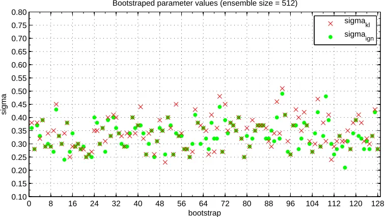
3.2 Resampled parameters for IGN/KL: For 128 samples, the ker-nel width σ minimizing KL-divergence (red crosses) is centered closely around 0.35. The σ that minimizes Ignorance (green dots) oscillates around the same value, supporting the suggestion that minimization of
Ignorance implicitly leads to minimization of KL-divergence. . . 99
3.3 Resampled parameters for IGN/KL:A different view of the result in Fig 3.3. For each ensemble size, we plot all 128 samples ofσminimizing both the Ignorance (blue) and KL-divergence (red). As the ensemble size
increases the two sets ofσconverge.. . . 99
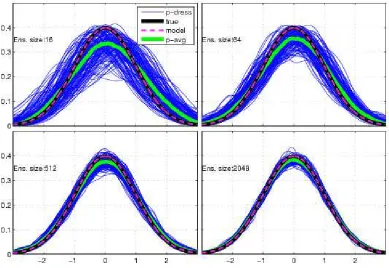
3.4 Gaussian PMS: The model (magenta dashed) as well as the system (black) areN(0,1) distributions. Both KD probabilities (blue dots) and their average (green dots) over 128 samples converge to the system
3.5 Bias and variance in PMS:Both bias (red) and variance (blue) quickly decay as the ensemble size (the horizontal axis) increases. Note that bias is measured as the expected value of the distance between the green and the black lines of Fig 3.4. . . 102
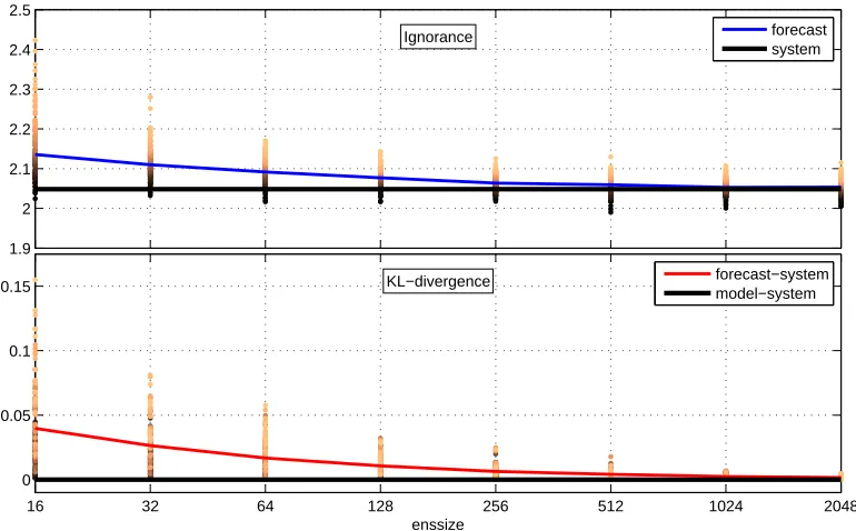
3.6 Ignorance and KL distance in PMS: Under PMS, increasing the size of an ensemble brings the forecasting density produced by kernel
dressing closer to the system density. The 128 sample average of
KL-divergence (red line) converges to zero, while the ignorance (blue line)
approaches the ignorance obtained by using probabilities assigned by the
system itself, i.e. the system defines a zero skill reference (black line). . . 103
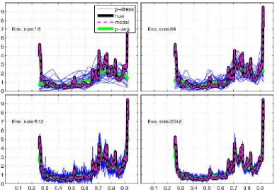
3.7 Logistic map PMS:The mean (green) of 128 estimates (blue) gradu-ally converges to the underlying density of the Logistic map (black) as
ensemble size is increased. Pseudo-likelihood type of kernel density
es-timation was used to construct the underlying density. The climatology
and the forecasts were obtained by iterating the set of initial conditions
using the Logistic map 1,000 times. . . 105
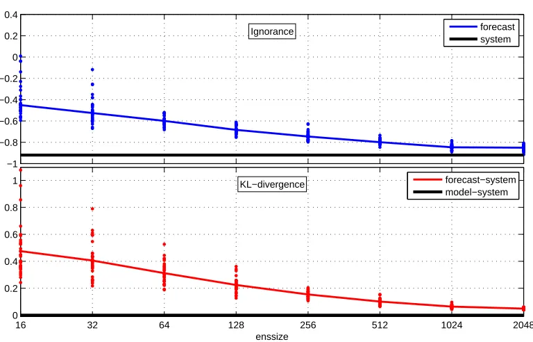
3.8 Ignorance of Logistic map PMS:Similarly to Gaussian PMS, both the Ignorance and the KL-divergence decrease significantly with the size
of ensemble. Due to the large second derivative of the underlying density,
the KL-divergence is rather high at small ensemble sizes when compared
to the Gaussian case. The maximum skill level is defined by the system
density, similarly to Fig 3.6. The maximum skill in terms of Ignorance is
3.9 Increasing the archive: For the ensemble size of 16 members, the size of forecast-verification pairs is gradually increased (doubled at each
step). For a given archive size Ignorance values are calculated using 128
samples. For small archive sizes, e.g. 16, the Ignorance values are widely
dispersed. Increasing the archive size produces more stable estimates.
The median value (green line) of the Ignorance also decrease, as the
archive size increases. . . 107
3.10 Increasing the archive: Each block shows same information as Fig: 3.9 but for a different ensemble size. A given block represents a given
en-semble size stated on the x-axis. Within a block there are 9 different
archive sizes and for each size 128 samples are generated and evaluated
by Ignorance. . . 108
3.11 IMS - System larger variance then model: Similar to Fig: 3.4 but outside PMS. The model produces ensembles with lower variance
that the system distribution. KD easily accommodates by increasing the
bandwidth and the forecasting densities quickly uncover the system density.109
3.12 IMS - System larger variance than model: The Ignorance of the model (top panel) is rather flat but decreasing. Note the scale of the
fig-ure, the model Ignorance (blue) is very close to the system (black). The
KL-divergence (bottom panel) decreases as KD utilizes more ensemble
members. Also KL-divergence is very close to its potential for all
en-semble sizes as KD very efficiently adjusts the bandwidth even for small
3.13 IMS - System smaller variance then model: Same as in Fig: 3.11 but this time the model produces ensembles with larger variance then
the system distribution. KD fails to recover the system distribution as
it cannot find bandwidth that would produce forecasting distributions
close to the system. . . 111
3.14 AKD - System smaller variance then model: The overdispersive-ness of the model (magenta) seems to be corrected by the AKD. The
forecasting densities (blue) closely surround the system density (black).
The size of the forecast archive is 2,048, the ensemble size is 512. . . 112
3.15 Forecast distributions: The punter uses the ensemble members (blue dots) to construct her estimate (blue curves) of the true
den-sity (red curves) governing the outcomes (red crosses). The house
constructs its estimate (magenta curves). . . 115
4.1 Forecasting sine function: DC correctly identified analogs within the training set (red), as demonstrated by the perfect forecast
(green/blue) at different initializations. All ensemble members,
at all leadtimes and initializations of the testing set (light red), lie
on top of each other and on top of the forecasted target. . . 140
4.2 Noisy sine forecasts: Adding noise to the sine function makes it more difficult for DC to identify analogs. Compared to Fig: 4.1,
the ensemble forecasts (blue/green) are no longer perfect. This is
4.3 Detail of noisy sine forecast: A detail of a single initializa-tion of the DC forecast (blue) showing the ensembles growing with
leadtime. Beyond leadtime 6, the pruning method starts being
ap-plied, keeping the ensemble size at 64. The initial ensemble is of
size 4, we observe 2 groups of 2 ensemble members very close to
each other at leadtime 1. . . 142
4.4 Pendulum in periodic (non-chaotic) regime: The left panel shows a phase plot of the FDP at a stable non-chaotic regime. The
system trajectory displays periodic behavior. The Poincare section
on the left shows only a small number of discrete points, a clear
sign of periodicity. The parameter values are: ωF = 2/3, b = 2
and g= 1. . . 144
4.5 Pendulum in chaotic regime: The phase portrait (left) reveals a very complex structure. The Poincare section (right) also show
a complex pattern suggesting a chaotic behavior. The parameter
values are: ωF = 2/3, b= 2 and g= 1. . . 145
4.6 DC forecasts of pendulum: For consecutive initializations of the DC forecasts (alternating blue/green) of the angular velocity
(light red) of FDP in the chaotic regime. Three of the four
dis-played forecasts successfully capture even a rather complex
behav-ior (peaks/troughs) up to 2/3 of the maximum leadtime, L= 30. The initialization at t = 1.57 (green) performs poorly relative to
climatology.. . . 146
4.7 DC forecast detail: Detail of the first initialization displayed in figure 4.6. The nonlinearities of the system cause the ensemble
forecasts to spread out. The growth of an ensemble is apparent
4.8 DC Ignorance in pendulum: Ignorance of the DC forecast rel-ative to climatology. The zero line (black) defines zero skill
refer-ence, i.e. skill of the unconditional climatology in this case. For a
model to outperform climatology, the relative Ignorance must be
below the zero line. The DC forecast displays a good forecasting
performance up to leadtimes 15-18. Beyond that, the climatology
takes over. . . 148
4.9 DC density in pendulum: Forecasting densities of the DC en-semble forecast. Selection of five different initializations of the DC
forecast are shown. At the initial leadtimes the densities are sharp,
with increasing leadtime they spread out as DC loses forecasting
performance. . . 149
4.10 DC Probability plumes (pendulum): The orange to yellow patches represent probability plumes of the DC forecast. Each
patch of color is a contour of a given percentile of a forecasting
distribution. The contours are created by connecting a given
per-centiles values over all leadtimes. Note that the perper-centiles of
cli-matology (light blue) are not changing; this is because we deploy
unconditional climatology, which does not change over time. Also
note that at long leadtimes the plumes of DC coincide with
cli-matological plumes. This is because DC forecasts lose skill and
climatology takes over, i.e. the blending parameterα= 1. . . 150
4.11 Varying DC parameters (Nino34): Parameters of the DC are varied and the resulting DC forecasts are evaluated relative to
4.12 DC Ignorance in Nino34: Three initializations of ENSEMBLES and DC forecasts evaluated relative to climatology. The August
initialization shows a poor performance by the LFPW and IFMK,
while the DC outperforms both. The ECMWF is the best
per-former in all three initializations. The overall performance of the
DC is comparable (or better at points) with the ENSEMBLES. . . 155
4.13 DC Ignorance of the ‘long run’ in Nino34: Same as in Fig 4.12 but for November initialization. The ECMWF is the
best overall performer although at leadtime 1 the DC outperforms
all the ENSEMBLES models. The DC, IFMK and LFPW models
maintain forecasting skill up to leadtime, 5 EGRR up to leadtime
7, and ECMWF considerably longer (up to leadtime 10). There
seems to be an improvement in performance toward the final
lead-time for all ENSEMBLES models. . . 156
4.14 Ignorance relative to DC in Nino34: Same as Figure 4.12 but here ENSEMBLES is evaluated relative to DC. Above the zero
line a model’s performance is worse then that of DC. The DC
is significantly outperformed only by ECMWF and EGRR in the
February initializations and at long leadtimes of the August
initial-izations. For the August initialization the DC outperforms IFMK
and LFPW. Overall, the DC performs comparably to ENSEMBLES.158
4.15 The ‘long run’ ignorance relative to DC in Nino34: Same as in Fig 4.14 but for the November initialization. Similar conclusion
emerges; the DC is significantly outperformed by only ECMWF
and EGRR models at leadtimes 3-7. For all other leadtimes and
4.16 Ignorance of the monthly climatology: Nino34: The Igno-rance of forecasts of monthly climatology shows that some months
are more difficult to (climatologicaly) forecast. January and March
are the most difficult months; April is rather easy, as the Ignorance
of -0.7 is much lower than the January/March Ignorance. A
possi-ble explanation of the forecast improvement for November
initial-ization is that the monthly climatology does not provide a strong
benchmark, so in relative terms the ENSEMBLES model forecasts
improve as the climatological forecast weakens. . . 161
4.17 Probability plumes of ECMWF model in Nino3.4: Per-centiles as given by the CDF of the ECMWF forecasts (red/yellow)
show the performance of selected November forecast initializations
in probabilistic terms. The plumes are plotted against a
back-ground of the plumes of monthly climatology (light blue). Note
how the climatological plumes vary with leadtimes. This is due
to monthly climatology changes with leadtime. The time period
selected shows 2 large El-Nino events in 1972/1973 and 1976/1977.
The ECMWF forecast performs well in capturing the onsets but
also the offsets of the events (red with white rim). Note how the
plumes overlap; this is due to the overlapping of initialization of
one forecast with the end of the preceding forecast. . . 162
4.18 Probability plumes of DC in Nino3.4: Same as in Fig: 4.17 but for the DC forecasts (red/yellow). The DC does a good job
in forecasting the onset of both the 1972 and 1975 events. The
forecasting performance is reduced after leadtime 5, beyond which
4.19 DC Ignorance in MDR:ENSEMBLES and DC model forecasts evaluated relative to monthly climatology in the MDR region. The
ENSEMBLES model performs rather well up to leadtimes 4-5 at
all initializations. The DC forecast performs comparably to
EN-SEMBLES as was the case in the Nino3.4 region. . . 164
4.20 Ignorance of the ‘long run in MDR: The November initial-ization evaluated relative to monthly climatology. All the
EN-SEMBLES models perform poorly as they loose skill at leadtimes
2-3. The DC is the best performer as at leadtime 3 it still has an
advantage of 0.5 Bits over climatology. . . 165
4.21 Ignorance relative to DC in MDR:ENSEMBLES models eval-uated relative to DC. None of the models outperforms DC for in
any of the three (Feb, May, Aug) initializations. . . 166
4.22 The ‘long run Ignorance relative to DC in MDR:Same as in Fig: 4.21 but for November initialization. Since all models perform
poorly at this initialization, none are expected to outperform DC
significantly. This is indeed the case; moreover, the DC is the best
performer at leadtime 3. . . 167
5.1 Growth of computational intensity. The computational cost of least square solution in terms of CPU (blue line) is plotted along
with a theoretical computational cost, given by FLOPs, for
differ-ent sizes of aM×M square matrix. The growth of the computa-tional cost follows a power law, atM = 104 it takes 35 seconds to calculate the solution on a platform with Intel duo-core 2.4 GHz
processor and 8 MB of memory. IncreasingM may quickly render
6.1 ΨΦ collecting the forecasting errors: Within a learning set (gray solid curve), a core model is initialized with a single initial
condition (red) and produces forecasts (green dots) up to leadtime
l = t. The forecast is contrasted with verification (red) and the forecasting error (red arrow) is collected. The light red dots
repre-sent verifications of the testing set (gray dash curve). The symbols
ht,ht−1 and ht−2 represent information available at times t,t−1
and t−2.. . . 200
6.2 ΨΦforecast: Initialized with an observation at timet(red point), the core model Φ produces leadtime 3 forecast (green). The Ψ
cor-rector produces corrections (blue) which are added to the forecasts
to obtain final forecast (blue) of the yet unobserved states (light
red points). . . 202
6.3 Error collection in PC: A core model P produces leadtime 1 forecasts (green), which are then contrasted with the verifications
(red dots) to obtain forecasting errors (red arrows) used as input
to theC corrector. As in ΨΦ errors are collected within a learning set (gray solid curve). . . 204
6.4 Error histograms: The histogram of about 400,000 collected forecasting errors (top) is very similar to the histogram based on
the 4,096 subsampled errors (bottom). The inverse sampling
pre-serves the shape of the histogram. . . 207
6.5 Subsampled v. all errors: In another evidence of the inverse sampling preserving the distribution of the forecasting errors, the
qq-plot is concentrated around the 45 degree line, the tails are also
6.6 P C forecast: Core model P is initialized at timet(red point) of the testing set (gray dash curve) and produces leadtime 1 forecast
oft+ 1 (green line), which is then corrected (red arrow) to produce
P C forecast (blue dot). The core model is then initialized with the
P C forecast at t+ 1 to produce leadtime 1 forecast of timet+ 2, which is then again corrected. The procedure is repeated as many
times as required to obtain a leadtimeLforecast. In this schematic
L= 3. . . 209
6.7 Lorenz84 forecasts: From top to bottom, PMS, non-corrected core model Φ, PC, ΨΦRBF and ΨΦLSQ forecasts of a selected
100-hour-long segment of the Lorenz84 system. P C outperforms the
other 4 (imperfect) models. The ΨΦLSQ quickly resorts to
fore-casting the mean ofx, the non-corrected Φ model loses skill after 20 hours. The ΨΦRBF marginally improves in this particular forecast. 212
6.8 lorenz63 Forecasts: Same models as in Fig: 6.7, used here to generate forecasts of x variable of the lorenz63 system 10 seconds ahead. The non-corrected model loses skill after 1.5 seconds. P C
performs very well, while ΨΦLSQ converges to mean rapidly. . . . 213
6.9 Ignorance evaluation of Lorenz84. Based on Ignorance the best performer of the 4 imperfect models is the P C (blue) fol-lowed by ΨΦRBF (magenta). Both the non-corrected Φ model and
ΨΦLSQ quickly lose forecasting skill beyond leadtime of 2-3 days.
6.10 Ignorance of Lorenz63. Similarly to Fig 6.9, the P C model (blue) delivers a significant improvement. ΨΦRBF (magenta)
im-proves the core model forecast (green) only marginally, while ΨΦLSQ
(orange) degrades the core model forecasts, possibly due to
over-fitting. . . 217
6.11 Lorenz84P C v. ΨΦ. Ignorance of theP C relative to ΨΦ (blue) shows that beyond the leadtime of 15 days theP C is outperforming the ΨΦ. Despite initial underperformance (up to 10 days), theP C
gains a great advantage of up to 1 Bit between leadtimes 45 to 100 days over ΨΦ. Note that below the zero line,P C outperforms ΨΦ. 218 6.12 RMS Lorenz84. The RMS of the ensemble mean is plotted
against leadtime for the 5 model forecasts of Lorenz84. Based
on the RMS the forecasting performance of the P C appears com-parable to the PMS, a result that is completely incorrect as the
PMS is by definition far superior model to theP C. . . 220
6.13 RMS Lorenz63. At the long leadtimes beyond 5.5 seconds the RMS evaluation rates ΨΦLSQas the best model, between leadtimes
6 and 8 even comparable to the PMS, an incorrect conclusion since
PMS must, by construction, outperform ΨΦLSQ. . . 221
6.14 Impact of number of centers on P C (Lorenz84): The core model complexity is increased by gradually increasing the number
of centers from 32 to 64 and 128 (green shades). The performance
of the core model improves with the complexity; the model with 128
centers has up to 0.8 Bit of advantage over the 32 center version
at leadtime 5. The performance of the P C is insensitive to the
6.15 Impact of number of centers onΨΦRBF (Lorenz84): Similar
to Fig: 6.14 but here ΨΦRBF is studied. Increasing the complexity
of the core model leads to a marginal improvement of ΨΦRBF
forecasts. For the core model with 128 centers ΨΦRBF slightly
outperforms the less complex versions between leadtimes 15-30 days.225
6.16 Impact of dataset size onP C (Lorenz84): The short dataset (see Appendix C.1) is used to perform core model and P C fore-casts. The complexity of the model is varied by using M =
{128,256,512,1024} centers; more centers can be afforded due to the lower dataset size. The core model performs much better then
in Fig: 6.14. The version with 1,024 centers is comparable to the
performance of theP C. TheP C is robust and delivers significant improvements for the low complexity models. . . 227
6.17 Impact dataset size. Comparison of computational intensity of
P C and ΨΦ. Considering ΨΦ with 1,500 errors available at each leadtime. To train ΨΦ for 163 leadtimes takes about the same time
as solving P C system for all leadtimes with 8,192 centers. 8,192 centers yields much better surface description than 1,500 centers
of the ΨΦ. Moreover P C with 8,192 is fully trained by the time
ΨΦ is in the middle of the training process. . . 229
B.1 Probability plumes of ECMWF in Nino3.4: Same as in Fig: 4.17 but here we show all forecasted time periods. Note the
difficult-to-forecast events of 1975-1978, 1981-1983, 1996-1998 . . . 242
C.1 Mutual information: Mutual information of Lorenz84 system for delays of up to 35 days of system time. The first local minimum
is detected at the delay of about 4 days, indicating an optimal delay
for the embedding of the timeseries. . . 247
C.2 Mutual information v. sample rate: This figure demonstrates how the embedding optimal delay depends on the sampling rate of
the system. The relationship is linear as sampling at higher rates
requires longer delays. . . 248
D.1 Computational intensity of least squares. This figure has been used in Section 5.1.2. For a square matrix of sizeM×M we plot the CPU time (blue) and number of FLOPs (green) required
to calculate a least square solution for different values ofM. While it takes about 5 seconds to calculate LS solution for matrix with
M = 5×10³, it takes about 35 seconds when the size is doubled.
The computational cost follows a power law. . . 255
D.2 Extrapolation of computational cost. Similar to Fig D.1 but for extrapolated values. Solving an exactly determined system for
datasets used in our work would take about 10 days. The values
were extrapolated using the linear relationship between the log-log
values plotted in the left panel.. . . 256
D.3 Impact of number of centers: Similar to Fig: D.1 but for an overdetermined system whereN = 4×10⁵ and varying number of centers M. Solving overdetermined system for the dataset size of
N = 4×10⁵ and 128 centers takes up to 25 seconds, a moderate
D.4 Cost for large number of centers. We use similar extrapolation as in Fig D.2. To solve a system for a dataset of sizeN = 4×10⁵
and M = 8,192 centers takes up to 4 hours of CPU time on our
platform. Beyond 1,024 centers the problem becomes intractable
Properties of Kernel Dressing
a - scaling parameter in Affine Kernel dressing
α - blending parameter between two densities
c(·) - density of a house (betting)
f(·) - punter forecasting density
G(·) - rate of growth
H(·) - Shannon’s entropy
IGN - Ignorance
k - index of an outcome (a density bin)
K - number of discrete outcomes (density bins)
KL - Kullback-Leibler divergence
l - forecasting leadtime
µ - expected value of a distribution
M - ensemble size
N - number of observations
N(·) - normal distribution
o - offset parameter in Kernel dressing
p(·) - model forecasting density ˆ
p(·) - estimate of model forecasting density
q(·) - system density
σ - bandwidth of a kernel or standard deviation of a distribution
sk - k-th outcome
θ - parameter vector
o(·) - odds issued by a house
t - time
τ - time delay
v(z) - variance of transformed ensemble
Vt - wealth at time t
Wk - number of occurrences of k-th outcome
xt - initial condition or an observation (potentially noisy)
yt - verification (potentially noisy)
Dynamic climatology and its benchmarking utility
b - damping friction (pendulum)
d - dimensionality of feature space (length of feature vector) ∆xa - difference of an image and analog
θ - angle between two vectors
DE - Euclidean distance
g - external forcing (pendulum)
K0 - number of analogs to be selected at leadtime 1
K - number of analogs to be selected beyond leadtime 1
l - forecasting leadtime
m - number of RBF centers
M - size of an ensemble
N - number of observations
ωF - forcing frequency (pendulum)
t - time
τ - time delay
w - phase window
xt - initial condition or an observation (potentially noisy)
xt - d-dimensional feature vector xa
t−τ - analogous feature vector xa
t−τ - analog of an observation xi
t−τ+1 - image of an analog
ˆ
Forecasting with Radial Basis Functions
A - distance or RBF matrix
Bj(·) - j-th basis function
c - center
c - vector of centers
d - dimensionality of observation point
f - system function ˜
f - estimate of system function f λj - j-th basis function coefficient λ - vector of basis function coefficient
M - number of centers
N - number of observations
φ - radial function
r - distance ind-dimensional space
t - time
x - d-dimensional observation point
Forecast correction PC v. ΨΦ
d - dimension (embedding dimension)
ε - forecasting error
ǫM - systematic part of a forecasting error, model error ǫ - stochastic part of a forecasting error
l - forecasting leadtime
L - maximum leadtime
K - size of a forecasting ensemble
M - number of RBF centers
N - size of data
t - time
τ - embedding time delay
xt - initial condition or an observation (potentially noisy)
xt - ensemble of initial conditions xt+l - ensemble forecast at leadtime l
˜
xt - ‘true’ system state ˆ
xt - forecast at time t
Introduction
Weather events [1, 96].
Probabilistic forecasting deploys Monte Carlo experiments [3, 56, 70], to pro-duce a collection (ensemble) [78, 93, 98, 103, 143] of multiple point forecasts by using slightly different initial conditions [69, 93, 143]. Building on the ensemble of forecasts, probabilistic methods can be used to assign probabil-ities to future outcomes, yielding forecasting distributions. The forecasting distributions express uncertainty about future evolution of a system. Proba-bilistic forecasting is in stark contrast with point forecasts, where a forecast is given in terms of an expectation and hence much less information, if any, regarding uncertainty is provided.
Any forecasting process, probabilistic or not, typically involves several stages, including:
• data retrieval and transformation,
• current state estimation,
• forecast formation,
• post-processing,
• forecast evaluation
• benchmarking.
Probabilistic approaches introduce additional challenge due to the fact that they work with forecasting distributions as opposed to expectations. In this work we focus on three particular steps of the forecasting process, all of which will be studied within the probabilistic context. The steps of our interest are:
2. evaluation
3. benchmarking
The three above steps enter the forecasting process after the forecast forma-tion. Our focus is therefore on improvement and understanding of the value of a forecast and not on forecast formation. In this thesis the value of a forecast is the common thread linking the three areas of our interest.
Error correction
Since all models are wrong [12] every forecast is prone to systematic errors. Error correction is a part of the post-processing stage and is designed to add additional value to a forecast by detecting and correcting systematic errors. If systematic errors are present it may be possible to detect and, to some extent, correct them [61, 99]. While simple error correction approaches focus on bias correction, more complex correctors may take the form of a two-stage procedure deploying an additional modeling layer on top of the forecasting model. In this thesis we deploy a two-stage procedure where the second stage corrector is designed to ‘learn’ the systematic errors of the first stage model and correct the errors in an iterative manner. The corrector is based on radial basis functions (RBF) [39, 40] and is shown to significantly improve forecasts for models with medium-to-large systematic errors while not de-grading performance of models with very low systematic error. Deployment of RBF as the corrector introduces some computational issues, relating the ‘power’ of the available computational device to the quality of the corrector. A critical discussion of the computational issues is also presented.
Evaluation
i.e. what is being scored, are of crucial importance if one aims to achieve a meaningful understanding of the value of a forecast. For point forecasts the frequently used score is the Root Mean Square Error (RMSE) and the object to score is the value of the point forecast. A similar approach is often adopted in probabilistic setting when some distance metric, e.g. RMSE, is applied to each of the ensemble forecasts (or their mean or other statistics). While such an approach could yield some intuition as to ‘how far’ the ensemble forecasts are from the target, it is questionable whether we would gain a real insight regarding the value of the forecast. The issue is that both RMSE and the individual ensemble forecasts only hold information about expectations, and disregard the very useful information contained within the dis-tribution of the ensemble forecasts. To make use of all the available information captured by an ensemble, the ensemble forecast must be trans-formed into a forecasting distribution, [15, 58, 112, 113, 115, 116] and the forecasting distribution itself then becomes an object of the scoring. There are two immediate challenges related to the process. First, what method should be used in order to transform the ensemble forecast into a distribu-tion and is the method statistically sound? Second, what score should be applied to the forecasting distributions?
Entropy [124] and Kullback-Leibler divergence [74]. By exposing the links among the three measures we hope to further highlight the usefulness of Ignorance as a probabilistic scoring rule.
Benchmarking
The real value of a forecasting model can only be understood on a relative basis, i.e. when compared to an alternative model (benchmark) [4, 48, 53, 156]. Benchmarking can thus be considered as an interpretation of the score of a forecast. In probabilistic setting, the output of a benchmarking model is transformed into distributions so that they are comparable to the forecasting distributions of the forecasting model. The benchmarking distributions often take very simple form, e.g. unconditional distribution of past observations (climatology). While simple benchmarks are often robust, they may lack performance. More complex benchmarks may be required to improve on the performance and thus become a ‘stronger’ benchmark. One way of creating a stronger benchmark is to construct conditional distributions. Conditioning on some event (e.g. month of a year in seasonal forecasting) may yield improvements in performance at an affordable cost of a moderate reduction in robustness.
project [28, 29, 36, 57, 152].
Thesis structure
This thesis is structured as follows: In Chapter 2 we provide background information that is drawn upon throughout the thesis. We discuss funda-mental concepts such as ensemble forecasting [78, 98, 143], forecasting sce-narios [65, 66] and sources of uncertainty [31, 131, 132]. We also define the concept of a forecasting framework, discuss methods of forecasting density construction [15, 58, 110] and (un)conditional climatological forecasts.
In Chapter 3 we investigate the properties of Kernel Dressing (KD) [15, 58], a method of transforming ensemble forecasts into forecasting densities, and study the properties of Ignorance [14, 49, 115], a measure of forecasting skill. We show that, although similar in concept, KD substantially differs from Kernel Density Estimation as understood by [11, 20, 129]; a fact that has not been fully recognized. We show analytically that minimizing Ignorance implicitly leads to minimization of Kullback-Leibler divergence [75]. We nu-merically demonstrate that under the perfect model scenario (PMS) [133], KD recovers the system density, suggesting that KD is an unbiased estima-tor. We also perform a novel numerical analysis of the KD properties outside PMS and demonstrate that caution must be exercised when deploying Affine KD (an extended version of KD), a new fact that has been previously over-looked [14]. Using the Kelly betting framework [72] we clarify important links between Ignorance and alternative Information theoretical measures, namely Shannon’s entropy [124–126] and Kullback-Leibler divergence.
constructing DC is that traditional zero skill references such as climatolog-ical forecast (climatology) may not yield lead an adequate quantification of model skill [53, 68, 89]. By defining a stronger reference, e.g. DC, we may obtain a more thorough understanding of the value of a forecasting model. We construct DC to outperform climatology and demonstrate that DC indeed does outperform climatology. We also construct DC to accommodate for degradation of forecasting skill at long leadtimes and to be capable of producing ‘new’ values, not contained within the training set. We deploy DC to forecast Sea Surface Temperatures over two regions important for seasonal weather forecasting: the Nino3.4 and the Main Development Region. We contrast the DC forecast with those of EN-SEMBLES models [36, 57, 152] and demonstrate that DC is a comparable, and occasionally a ‘better’, performer.
In Chapter 5 we provide background information on radial basis functions (RBF), as they are extensively used in Chapter 6. We discuss the basic setting of RBF interpolation and approximation, and give arguments for formulating forecasting problems in terms of RBF approximation.
In Chapter 6 we present predictor-corrector (P C), a new approach to im-proving the forecasts of an imperfect model, based on iterative corrections of the systematic part of a model error [61, 67, 137]. For several nonlinear systems, we show the P C significantly improves imperfect model forecasts and is superior to an alternative approach of ΨΦ [62, 63].
maintains its superiority at medium range, even in settings with a (much) more skillful imperfect model. The computational aspects of theP C and ΨΦ approaches are also discussed in detail, both in general and specific terms.
Background
This thesis capitalizes on a number of concepts of statistics, information theory and dynamical systems. In this chapter, we provide background in-formation that will be drawn upon throughout the thesis.
We begin with a general description of a forecasting problem in Section 2.1. We discuss a system, a forecasting model, and give our definition of a forecast-ing framework. We follow with a discussion of forecastforecast-ing scenarios [65, 66] and briefly describe sources of uncertainty [31, 131, 132] obscuring the future evolution of a dynamical system.
In Section 2.2 we provide a brief description of ensemble forecasting [78, 98, 143] and discuss several methods of forecasting density construction [15, 58, 110]. Both ensemble forecasting and forecasting densities are key concepts in probabilistic forecasting and will be used throughout this work. We also define unconditional and conditional climatological forecasts and discuss their application. These climatological forecasts are used extensively in Chapters 4 and 6
of forecasting density construction and evaluation. We discuss the general aspects of forecast evaluation in Section 2.4, where we also define Kernel dressing [15].
At the center of forecast evaluation are measures of forecasting performance. Measures originating from Information theory [22, 72, 74, 124, 125] have proved to be of particular importance [46, 115]. The Information theoretical measures and their importance for evaluation of forecasting performance are discussed in Section 2.3.
Lastly, we briefly discuss issues related to seasonal weather forecasting and describe the forecasting models of the ENSEMBLES project [36, 57], as they will be a subject of study in Chapter 4.
2.1
Forecasting
The future evolution of any physical system is clouded with uncertainty, which limits our ability to precisely determine future states of the system. In our efforts to better understand the behavior of a system, we construct inherently imperfect mathematical models describing the underlying rule gov-erning the system. These imperfect models are often used to issue statements about future system states - a process called forecasting [5].
In forecasting, systems are often classified as eitherdeterministic or stochas-tic. Deterministic systems are governed by a fixed behavioral rule and do not involve any randomness. Stochastic systems, on the contrary, do involve random behavior, although their behavioral rule may also involve a fixed (non-random) part.
sys-tems, a subclass of deterministic systems. A good definition of a dynamical system can be found on Wikipedia [155]: a dynamical system is ‘a mathemat-ical concept where a fixed rule describes the time dependence of a point in a geometrical space’. An example of dynamical systems are physical laws, typ-ically described in terms of differential equations, e.g. a simple pendulum[8] derived from Newton’s second law
Aθ¨=−gsinθ (2.1)
where A is the length of the pendulum,θ is the angular displacement of the rod and g is gravitational force.
In our work (e.g. Chapter 4), we apply probabilistic methods in the context of weather forecasting. While the pendulum system of Eq. 2.1 is an example of a simple dynamical system, weather is an example of a very complex dynamical system. Weather is defined as a state of the atmosphere, and is often described using a set of fixed behavioral rules, i.e. physical laws such as the one in Eq. 2.1, which form a dynamical system. Weather is also considered a chaotic system [81]. A chaotic system is a type of dynamical system sensitive to initial conditions. Given two initial states that are very close (as quantified by some measure), the future states obtained by evolving the two initial states may end up very far from each other. In other words, small differences in initial states (conditions) may yield entirely different forecasts. Obtaining a useful forecast of complex, chaotic system such as weather is a challenging task. Yet due to its direct impact on many fields, including agriculture, transport, insurance, etc., weather forecasting is of crucial importance.
fields as well as industries and is applied to a large variety of dynamical and stochastic systems differing in complexity as well as their nature (natural vs. mathematical). It is not possible to apply our approaches to all possible classes of systems; there are simply too many of them. What we can do is apply our methods to a few selected systems for which we believe our ap-proaches are useful. Our applications therefore involve simple mathematical dynamical systems (e.g. Lorenz63 [81], pendulum) but also a highly complex chaotic system (weather).
Although we deliver a number of results that may help to better understand the studied systems (or their models), our main goal is to present probabilis-tic methods and how they may be applied in forecasting. Our emphasis is not on system analysis, but rather on a thorough description of (new or ex-isting) probabilistic methods and their properties, as well as a comprehensive illustration of their application.
2.1.1
System model pair
Forecasting a system requires a vehicle, aforecasting model. By a forecasting model, we will understand a mathematical description of a system. Models are constructed to describe systems, and so the models themselves can also be classified as deterministic and stochastic. To describe a dynamical system, a physicist would typically use a deterministic model, i.e. differential equation (or a set of equations) similar to Eq: 2.1. On the other hand, a statistician would probably choose a stochastic model to describe the system. In this work, we will be using both approaches.
equa-tions describing the same system. The obvious reason for having more than a single mathematical description of a system is that it may be impossible to describe the system exactly. In fact, no model of a physical dynamical system is able to exactly describe the system at hand, simply because forecasters do not possess a perfect knowledge of all laws occurring in nature.
2.1.2
Forecasting framework
The process of forecasting involves several stages, the collection of which we call a forecasting framework. Although the number of stages may vary with an application, in general, the forecasting framework involves:
(1) collection of observations,
(2) data quality control,
(3) current system state estimation,
(4) forecast generation,
(5) forecast post-processing,
(6) construction of forecasting density,
(7) forecast evaluation.
observation devices every 12 hours. To collect and quality control such an amount of data is a major task.
Collected and quality-controlled data then may serve as an input for current state estimation procedures. In nonlinear dynamical systems small errors in a current state estimation may ruin a point forecast as chaotic (or highly nonlinear) systems, such as weather, display high sensitivity to initial con-ditions [79, 81]. Due to the significant impact on the quality of a forecast, state estimation methods, such as 4DVaR [139, 142], Particle Filter [50, 108], Gradient Descent [59, 64] etc., are a very active area of research.
Forecast generation is a central part of the forecasting framework. The fore-casting model is initialized by initial conditions determined within the state estimation stage. The initial conditions are than integrated by the model to produce a raw ensemble of point forecasts for a required future time, which we call a leadtime.
The raw ensemble often contains biases. Model output post-processing is a type of quality check applied to the ensemble and designed to remove biases. Outliers may also be handled within this stage.
If a probabilistic forecast is to be issued, the post-processed ensemble needs to be turned into a forecasting PDF, which assigns probabilities to possible future states of the forecasted system. The forecasting PDFs are also used in the forecast evaluation to ex-ante assess the rate of success of a forecast.
frame-work.
2.1.3
Perfect and imperfect model scenario
When investigating properties of a forecasting model, both thePerfect model scenario (PMS) [65, 133] and the Imperfect model scenario (IMS) [66, 133] are useful concepts. In Chapter 3, we rely on PMS to demonstrate properties of a forecast evaluation method. To explain what we understand by PMS, we first describe IMS and than define PMS as somewhat the opposite of IMS. The descriptions loosely follow [133].
Imperfect model scenario: IMS is a scenario in which the forecasting
model provides an imperfect description of a system. It assumes that a forecaster does not know the system rule exactly. Often it is also assumed that the system’s current state is not known exactly.
Every ‘real world’ forecasting exercise is an example of IMS; there are no perfect models in the real world. A physicist does not know exactly the governing equations of a particle motion, a weather forecaster has at best a crude description of a weather system and no social scientist has a model that would perfectly predict an election outcome. Under IMS the forecasting model always produces an imperfect forecast.
Perfect model scenario: PMS is the opposite of IMS to some extent.
Consider a forecaster with a complete knowledge of the laws governing a sys-tem. This perfect knowledge allows him/her to construct an ideal description of a system, a perfect model.
dynamical system, a forecaster needs to know exactly the current state of a system. Any uncertainty about the current state due to an observational error, or any other source of uncertainty, accumulates over time [98, 132, 133] leading to an imperfect forecast. Under PMS, a forecast is always imperfect unless the exact current state is known.
With real world forecasting exercises falling under IMS, is there any example of PMS? The answer is that PMS can only be constructed. This can be achieved by letting the model act as both the model and the system. Con-sider a forecasting model taking the form of a standard normal distribution,
N(0,1), and a system producing a sample from the same distribution at each time t, i.e. xt iid
∼ N(0,1). The forecasting model will produce an imperfect but highly valuable forecast ofxt, since the distributions of the model forecast
and system states will be equivalent. This may look like cheating, but PMS is in fact an ideal testbed for understanding the properties of a forecasting model, as we show in Chapter 3.
Perfect ensemble: Often, it is useful to use the concept of a perfect
en-semble in combination with PMS. With a perfect ensemble, we assume a distribution of a current system state, which is a much weaker assumption than assuming an exact knowledge of a current state. The distributional assumption allows for sampling current state ‘candidates’, so that an en-semble of ‘perfect initial conditions’ may be constructed. Under PMS and perfect ensemble, a forecast remains imperfect, but the forecast distribution is equivalent to the distribution of the future system states.
eval-uation method; both the forecasting model and the current state estimation method may be ruled out as a sources of the bias. Without the perfect en-semble, the forecaster could not be certain whether it is the evaluation stage or the current state estimation stage causing the bias.
2.1.4
Sources of uncertainty in physical systems
Forecasts of any dynamical systems are inherently inaccurate. There are two major sources of uncertainty directly influencing the accuracy of a fore-cast [98, 99]: uncertainty about the current state of a system, i.e. the initial condition uncertainty, and uncertainty due to the inaccuracies in a forecast-ing model specification, the model error [61, 137].
Initial condition uncertainty: Under IMS conditions, uncertainty stems
from the forecaster’s inability to accurately observe a current state of a sys-tem, an observation error. The observation error is particularly influential when sets of differential equations are used as a model. It is well known [81], that for nonlinear (and in particular chaotic) systems/models, an arbitrarily small initial error in the initial state will accumulate (grow) over the forecast-ing leadtime. The error growth will eventually cause the forecasting model to reach its predictability limit [133], a leadtime beyond which the forecast is no longer ‘useful’. Although stochastic models may be less susceptible, they also may suffer from the imprecise determination of the initial condition.
Model error: The uncertainty related to the model formulation arises due
to an imperfect understanding (or description) of the predicted system. The imperfect model formulation leads to a model error, which will eventually cause the model to reach its predictability limit.
disen-tangling the model error is as follows:
(1) Structural error: The equations describing the systems are ‘incorrect’, i.e. there may be a variable missing or a function is incorrectly specified.
(2) Error due to a choice of approximation and discretization method: A forecasting model is often deployed on a computational device, which is by nature of a finite precision. i.e. a digital (discrete) device. Model equations describing a given system frequently take a continuous form. To deploy a model on a computer, the continuous equations need to be discretized. This transformation involves numerical methods that of-ten require approximations and truncations [145], and thus introduce ‘imperfections’ into the model’s original (analytical) equations. The choice of a transformation method influences the severity of imperfec-tions. A poor choice of transformation may lead to a significant model error, even in computers with very high precision.
may exhibit lower errors than those with high mesh density but poor approximation/discretization method.
To minimize the observation error, a forecaster may attempt to improve the measuring device. This, however, may prove difficult due to budget con-straints or the fact that the device is already state-of-the-art. A more real-istic approach is to use a number of observational devices and to determine the initial state as some function of their outputs. Alternatively, a fore-caster may attempt to sample the distribution of initial states as discussed in Section 2.2.1.
To address model error, a forecaster may attempt to obtain a better under-standing of the system. Another option is to see whether the model error contains a systematic part and if so to correct it. When using deterministic models, the systematic part of the model error is frequently present. In such cases, error detection and correction algorithms can be very successful in re-ducing the systematic part of the model error. We suggest a framework that deals with the systematic part of a model error in Chapter 6.
2.2
Probabilistic forecasting
2.2.1
Ensemble forecasting and forecasting densities
In Section 2.1.4, we have discussed how an inaccuracy in determination of a current state accumulates over the integrations of a forecasting model, and degrades the quality of a forecast. We have also mentioned that a forecaster may address the initial condition uncertainty using Monte Carlo methods.
sample of possible future states of a system.
To produce an ensemble forecast (or simply an ensemble), a forecaster sam-ples possible current states, generating M initial conditions xt = {xt,k}Mk=1,
which form an initial condition ensemble at the initial time t. The initial conditions xt,k are then iteratively input into a forecasting model to produce an ensemble of M point forecasts, ˆxt+1 ={xˆt+1,k}Mk=1, i.e., an ensemble
fore-cast at leadtime t+ 1. Fig: 2.1 shows a simple schematic of ensemble forecast generation, for the case of M = 4 initial conditions. In an ideal case, the forecast values would be a representative sample of the possible system states at time t= 1.
t=0 t=1
−5 0 5
observation verification
initial condition 1 initial condition 4
forecast 1 forecast 4 schematic of ensemble forecast
x
leadtime
Figure 2.1: Ensemble forecast: Using an observation (large red circle) at time
t= 0, an ensemble of initial conditions (small red circles at t= 0) is constructed and iterated forward using the model (blue lines) to obtain an ensemble forecast (small red circles at t = 1). At time t = 1 the forecast can be verified with an outcome (red cross), i.e. system state observed at time t+ 1.
Forecast-verification archive: A forecasting model is often used to
time, when the forecasted system states are actually observed, an archive of forecast-verification pairs may be formed. The archive is constructed sim-ply by pairing an ensemble with the observed system state at each leadtime. The archive of forecast-verification pairs can than serve as a training set when constructing forecasting densities and/or evaluating forecasting performance of a model.
Forecasting distribution: A natural way of describing an uncertainty is
via distributions. A sample of possible future states, an ensemble forecast, may be turned into aforecasting distribution, ˆp. The forecasting distribution is able to concisely summarize the uncertainty caused by observational and modeling errors. When producing forecasts forL >1 leadtimes, a forecasting distribution is constructed for each leadtime l, giving a sequence of distribu-tions {pt+lˆ }L
l=1. There are a number of methods to construct the forecasting
distributions, and we briefly discuss some of them in the next section 2.2.2.
An important question is: why would a forecaster wish to turn ensemble forecasts into forecasting densities? There are three main reasons for doing so. First, a forecasting density can be used to assign probabilities to the possible future states of the system. Second, a forecasting density enables evaluation of a forecast in probabilistic terms. This is an important part of the forecasting framework discussed in more detail in Section 2.4. Third, the density construction is often designed to include post-processing procedures such as bias correction, designed to improve raw forecasts ex post.
2.2.2
Constructing forecasting densities
There are number of methods to turn ensemble forecasts into forecasting densities. Here we briefly discuss a selected few, namely Logistic regression,
particular methods, we aim to provide insight regarding ensemble-based den-sity construction. Since our selection represents rather different approaches, we hope to demonstrate the diversity of existing approaches. We note that for this work, the most relevant is the Gaussian dressing, which provides a link to our preferred method ofKernel dressing (section 2.4.3). Although Logistic regression and Bayesian averaging are not directly linked to Kernel dressing, we hope that understanding the alternatives will help the reader to better appreciate the concept of density construction from ensemble forecasts. A detailed account of methods discussed, as well as alternative methods, can be found in [157].
Logistic regression: In weather forecasting, logistic regression has been a
frequent tool of forecasting density estimation [157] [54]. Logistic regression is a useful method when a forecaster takes an interest in the quantiles, q, of possible outcomes. In ensemble forecasting the logistic regression often takes the form of
P(y≤q) = 1 +exp(β0+β1¯x+β2σˆ)
exp(β0 +β1x¯+β2σˆ) (2.2)
where ¯xis a mean of an ensemble forecast, ˆσ is the ensemble variance andy
is the observed system state, i.e., the verification. The parameters β0, β1, β2
are determined by maximizing likelihood of the verification y being in the quantile q over all forecast-verification pairs contained within an archive.
Gaussian dressing: Gaussian dressing (GD) is a sort of ensemble
dress-ing a density construction method proposed by [116]. GD applies gaussian distribution to each forecast-verification pair and takes the form of
p(y;x) = √ 1
2πσ2e
−(x−µ)2
There are different ways of determining the parameters µ and σ. In the simplest form of GD µand σ are set to some function of the ensemble mean and ensemble variance respectively, i.e., µ =f(¯x) and σ = g(ˆσ). As noted by [14], this has the undesirable consequence that the forecasting distribution is solely based on the ensemble forecast, i.e. information provided by the actually observed state y is neglected. Other authors, e.g. [48, 58] suggested to determine µ and σ according to a forecasting performance. This leads to maximization of some function ofp(y) over the forecast-verification pair. We will discuss the performance-based approach in Section 2.4.3.
Bayesian model averaging: Bayesian model averaging (BMA) [110]
ad-dresses an uncertainty stemming from selecting a suboptimal model. Instead of relying on a single model BMA considers K candidate models and calcu-lates a posterior probability of an outcome by conditioning on the K models. Consider a model k producing a l step ahead point forecast xk,t+l, where xk
represents the k-th ensemble member. The forecast xk,t+l is associated with a PDF, qk(y|xk,t+l). The PDF qk is a PDF of the outcome y conditional on
xk being the best forecast in the ensemble forecast. Dropping thet+l term for simplicity, the BMA model can be written as
p(y|x1, . . . , xK) =
K
X
k=1
wkqk(y|xk) (2.4)
from the historical errors of the forecast xk.
2.2.3
Unconditional climatology and climatological
fore-cast
The climatological distribution, or simply climatology, is an unconditional distribution, pc(x), of observed values of a system variable x over the time period [t − ∆, t + ∆]. Climatology may be constructed using parametric or non-parametric density estimation methods. In our work, we estimate climatology using the Kernel dressing method described in Section 2.4.3.
Climatology is not only useful as a statistical description of the forecasted data, it may also be used as a simple probabilistic forecasting model. When used as a forecasting model, the forecasting density for a given leadtime l
simply coincides with the climatology, pt+l(x) =pc(x). This approach yields a probabilistic forecast that does not change over leadtime.
Assuming that the systems dynamics is (to some degree) captured by data used to construct climatology, the climatological forecast may be considered a robust forecast. In other words there will be a few surprises to the clima-tology if the dataset reasonably captures the system’s past dynamics and the dynamics do not change abruptly.
reference forecast?
Climatology may be constructed in a number of ways, e.g. via parametric density estimation [58], kernel density estimation [11, 129] or kernel dressing (see Section 2.4.3). The climatological distribution can be used to produce a very basic climatological forecast, simply by sampling a single (or multiple) value(s) from the distribution.
2.2.4
Conditional climatology
Climatological distribution may take more complex forms. We can construct so called conditional climatologies by conditioning on some feature of the data. For instance, when a seasonality is present, a forecaster may choose to condition on a particular season. In weather forecasting, it is common practice to construct amonthly climatology by conditioning on a month of a year. In economics, climatologies conditional on a business or political cycle are often used.
In Chapter 4 we will be using a monthly climatology to benchmark alternative forecasts. Monthly climatology is a special case of a climatology where we condition on phase information. In general, climatology conditioned on a phase can be defined as
pθ(x) =p(x|xt:t∈[t−θ1, t+θ2]) (2.5)
t would be set to the number indexing a given month and θ1 = θ2 = 0. In practice, one may construct monthly climatologies that span over more than 1 month by setting θ1 =θ2 >0. Asymmetric monthly climatologies can also be constructed by setting θ1 6=θ2.
We note that it only makes sense to construct monthly climatology when a monthly seasonality is actually present in the data. Constructing monthly climatology of temperatures over sub-Saharan Africa may not make much sense, since the seasonality at these latitudes may not be related to months but rather to seasons.
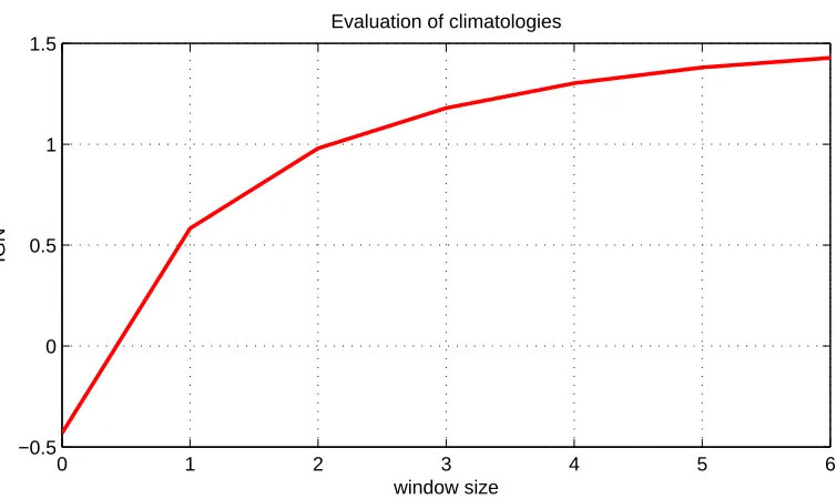
In the following sections we use data from the application in Section 4.3.2 to demonstrate how monthly climatology can be a more useful climatology than the unconditional. In Fig: 2.2 we show a measure of forecasting performance against the varying size of the phase angle. Since the data used to gener-ate the plot are monthly data, the phase angle has a simple interpretation. Window size of 0 corresponds to a ‘pure’ monthly climatology, i.e. only the same months are considered in the conditioning. Window size of 6 means that all months of a year may be considered, which leads to unconditional climatology. The measure of performance will be explained in Section 2.4.2; for now we can say that lower value mean a better performance. Clearly, the window size of 0, which corresponds to the ‘pure’ case of monthly climatol-ogy, gives much better results then the window size of 6 which corresponds to unconditional climatology.
2.2.5
Blending climatological and model forecasts
0 1 2 3 4 5 6 −0.5
0 0.5 1 1.5
Evaluation of climatologies
window size
[image:61.612.119.496.129.354.2]IGN
Figure 2.2: Climatological ignorance in Nino34: Forecasting performance of climatology of monthly SST temperatures over Nino3.4 region evaluated in terms of Ignorance. Ignorance is calculated for a varying size of a phase angle (window).
For window size of 6 the conditional climatology becomes unconditional, as all observations will fall within the window. The optimal window in this case is 0 (the lowest level of Ignorance), i.e. the climatology should condition only on a
given month of a year.
however, the error growth will cause a model forecast to deteriorate. Thus a forecasting model that performs well at short leadtimes may be outperformed by climatology at long leadtimes. The concept of blending aims to prevent the model from underperforming the climatological forecast.
The idea is simple. For a given leadtime, a model forecasting density pm(x) is ‘blended’ with the climatology pc(x) producing a ‘final’ forecasting density
p(x) =α×pm(x) + (1−α)×pc(x) (2.6)
where α ∈ [0,1] is a blending parameter. As a result, at leadtimes where the model significantly outperforms cli