Forecasting the geomagnetic activity of the Dst Index using radial basis function networks

This is a repository copy of Forecasting the geomagnetic activity of the Dst Index using

radial basis function networks.

White Rose Research Online URL for this paper:

http://eprints.whiterose.ac.uk/74600/

Monograph:

Wei, H.L., Zhu, D.Q., Billings, S.A. et al. (1 more author) (2006) Forecasting the

geomagnetic activity of the Dst Index using radial basis function networks. Research

Report. ACSE Research Report no. 941 . Automatic Control and Systems Engineering,

University of Sheffield

Reuse

Unless indicated otherwise, fulltext items are protected by copyright with all rights reserved. The copyright exception in section 29 of the Copyright, Designs and Patents Act 1988 allows the making of a single copy solely for the purpose of non-commercial research or private study within the limits of fair dealing. The publisher or other rights-holder may allow further reproduction and re-use of this version - refer to the White Rose Research Online record for this item. Where records identify the publisher as the copyright holder, users can verify any specific terms of use on the publisher’s website.

Takedown

If you consider content in White Rose Research Online to be in breach of UK law, please notify us by

Forecasting the Geomagnetic Activity of the Dst Index

Using Radial Basis Function Networks

H. L. Wei, D. Q. Zhu, S. A. Billings, and M. A. Balikhin

Research Report No. 941

Department of Automatic Control and Systems Engineering

The University of Sheffield

Mappin Street, Sheffield

S1 3JD, UK

Forecasting the Geomagnetic Activity of the Dst Index Using

Radial Basis Function Networks

H. L. Weia, D. Q. Zhub, S. A. Billingsc, and M. A. Balikhind

a,b,c,d

Department of Automatic Control and Systems Engineering, University of Sheffield, Mappin

Street, Sheffield, S1 3JD, United Kingdom

Email:

Abstract

The Dst index is a key parameter which characterises the disturbance of the geomagnetic field in magnetic storms. Modelling of the Dst index is thus very important for the analysis of the geomagnetic field. A data-based modelling approach, aimed at obtaining efficient models based on limited input-output observational data, provides a powerful tool for analysing and forecasting geomagnetic activities including the prediction of the Dst index. Radial basis function (RBF) networks are an important and popular network model for nonlinear system identification and dynamical modelling. A novel generalised multiscale RBF (MSRBF) network is introduced for Dst index modelling. The proposed MSRBF network can easily be converted into a linear-in-the-parameters form and the training of the linear network model can easily be implemented using an orthogonal least squares (OLS) type algorithm. One advantage of the new MSRBF network, compared with traditional single scale RBF networks, is that the new network is more flexible for describing complex nonlinear dynamical systems.

1. Introduction

from available observational data. In such a case, the solar wind parameters will be considered as inputs and the geomagnetic indices will be treated as the outputs of the magnetosphere system.

In the literature many types of model structures have been proposed for nonlinear dynamical systems identification, where the inner structure of the underlying system is unknown but only the input and output observational data are available. The NARMAX models, neural networks, radial basis function networks, neurofuzzy networks, and wavelet networks and wavelet multiresolution models are among the classes of the most popular model types (Leontaritis and Billings, 1985; Billings et al., 1989, 1998; Chen et al., 1990; Chen and Billings, 1992; Boaghe et al., 2001; Liu, 2001; Harris et al., 2002; Lundstedt et al., 2002; Wei et al, 2004a; Billings and Wei, 2005a, 2005b; Sharifi et al., 2006).

Radial basis function (RBF) networks, as a special class of single hidden-layer feedforward neural networks, have been proved to be universal approximators (Hartman et al., 1990; Poggio and Girosi, 1990; Park and Sandberg, 1991) for arbitrary nonlinear functions. One advantage of RBF networks, compared to multi-layer perceptrons (MLP), is that the linearly weighted structure of RBF networks, where parameters in the units of the hidden layer can often be pre-fixed, can easily be trained with a fast speed without involving nonlinear optimization. Another advantage of RBF networks, compared with other basis function networks, is that each basis function in the hidden units is a nonlinear mapping which maps a multivariable input to a scalar value, and thus the total number of candidate basis functions involved in a RBF network model is not very large and does not increase when the number of input variables increases.

This study aims to propose a new direct approach for identifying a mathematical model for the magnetospheric dynamics without any a priori information of the physical processes of the magnetosphere system but only a limited observational data. To achieve this objective, a novel class of RBF networks is introduced to represent the underlying dynamics of the magnetosphere system. Unlike a conventional single scale (kernel width) RBF, where all the basis functions have a common single scale, or each basis function has a single individual scale, the new RBF network uses a number of multiscale basis functions, where each basis function has multiple scale parameters (kernel widths). The new network will be referred to as the multiscale RBF network (MSRBF). The construction procedure of such a MSRBF network is as follows. The positions (centres) of the basis functions in the MSRBF network are initially pre-clustered and selected using some unsupervised clustering algorithm say the k-means clustering method. For each selected centre, the associated scales (kernel widths) are determined heuristically, and the selected centres and scales are restricted to a fixed grid. Finally, an MSRBF network is converted into a linear-in-the-parameters model form. A forward orthogonal

regression (FOR) algorithm (Billings et al., 1989; Chen et al. 1989;Wei et al., 2006), regularised by a

Bayesian information criterion (BIC) (Schwarz, 1978; Efron and Tibshirani, 1993), is then used to train the MSRBF network, and a parsimonious model, which consists of a relatively small number of regressors, is then used to predict the Dst index.

2. The linear-in-the-parameters representation

Consider the identification problem of a single-input and single-output (SISO) nonlinear dynamical system, for which N pairs of input-output observations,{u(t),y(t)}tN=1, are available. Under some mild conditions a discrete-time nonlinear system can be described by the following NARX model (Leontaritis and Billings, 1985)

) ( )) ( , ), 1 ( ), ( , ), 1 ( ( )

(t f y t y t n u t u t n e t

y = −  − y −  − u + (1)

where u(t) , y(t) and e(t) are the system input, output and noise variables;

n

unknown and needs to be identified from the available observations. It is generally assumed that e(t)

The central task of system identification is to find an efficient approximator fˆ for the nonlinear function f from the observational data. Several model types can be used to approximate the nonlinear function f and different model types often involve totally different training/learning strategies. One of the most commonly used methods is to approximate the nonlinear function f using a series of specified basis functions, whose local and global properties are known. One advantage of the basis function approximation is that the expression can easily be converted into a linear-in-the-parameters form, which is an important class of representations for nonlinear function approximation and signal processing. Compared to nonlinear-in-the-parameters models that usually involve complex and time-consuming nonlinear optimisation, linear-in-the-parameters models are simpler to analyse and quicker to compute and estimate.

Letd =n_y+n_u and x(t)=[x1(t),,xd(t)]with

    + ≤ ≤ + − − ≤ ≤ − = u y y y y k n n k n n k t u n k k t y t x 1 )) ( ( 1 ) ( )

( (2)

A general form of the linear-in-the-parameters regression model is given as

) ( )) ( ( ˆ )

(t f t e t

y = x + ( ( )) ( )

1 t e t M m m m + =

∑

θ = T(t) +e(t) (3)

where M is the total number of candidate regressors, φm( tx( ))(m=1,2, …, M) are the model regressors andθ_mare the model parameters, and (t)=[φ₁(x(t)),,φ_M(x(t))]Tand are the associated regressor vector and parameter vector respectively.

In the present study, a new multiscale RBF (MSRBF) network model with Gaussian kernels will be used to construct the approximator fˆ , and this is discussed in the next section.

3. Multiscale RBF networks

The multiscale RBF (MSRBF) network aims to accommodate both the local and the global properties of the basis functions by including both small and large scales (kernel widths) in the network in a hierarchical multiscale way. In the multiscale modelling framework, a set of scale parameters (multiple kernel widths) will be assigned to each basis function.

3.1 The Network Structure

Taking the case of single-input and single-output nonlinear dynamical systems as an example, the MSRBF network possesses the following structure

∑∑∑

∑

0 0 1

) , ( , , (RBF) , , 1 (linear) ) , ); ( ( ) ( )) ( (

ˆ _{x θ θ ϕ x c s (4)}

where θk(linear)and

(RBF) , ,jm i

θ are constants (unknown parameters), , , ( ( ); , (, ))

j i m m m j

i x t c s

ϕ is the mth Gaussian

basis function of the form

) , ); ( ( (, ) , , j i m m m j

i x t c s

ϕ                 − −         − − =

∑

∑

y n n

wherex(t)=[x₁(t),,x_d(t)], defined by (2), is the network input vector, c_m(t)=[c_m,1,,c_m,d] is the centre of the mth basis function, and the scale vector s( jmi, ) for the mth basis function in the network is

defined as ] , , , , , [ : 1 ) ( , ) ( , : 1 ) ( , ) ( , ) , (         u y n j m u j m u n i m y i m y j i

m = s s s s

s (6)

The number of the basis functions (or the number of centres) in the network isN , the number of c

scales for the output and input variables in the mth basis function is (I+1) and (J+1) respectively. Thus, for a single-input and single-output system, the network involves a total of M =(I+1)(J +1)Ncbasis

functions.

All given observations can be considered as candidate kernel centres providing that the observational data set is not very long. For a long data set, some unsupervised learning algorithms can be used to locate the centres of the basis functions in only those regimens of the input space where significant data are present, and supervised learning approaches can then be used to train the network

further. The details for the determination of the centres c and the kernel widths m

) , ( ji m

s are given

below.

3.2 Determine the centres

If the observed data set is not very long, all given observations can be considered as candidate kernel centresc . If, however, a long data set is involved and all the observations are still considered m

as candidate kernel centres, the initial MSRBF network will then include a great number of model terms and the training of the network will be time consuming. To overcome this problem, the well-known k-means clustering algorithm (Duda et al., 2001), coupled with the sum-of-squares criterion proposed by Krzanowski and Lai (1988), can be used to significantly reduce the number of candidate centres of the basis functions in the network. The sum-of-squares clustering algorithm is briefly described as below.

Assume that the data are given in the form of a matrix X of sizeN×p, with the ith row given by

the vector zi =[zi1,,zip] representing the observation vector of the ith object. The given N

observations can be partitioned into k groups (clusters), denoted by G1,G2,,G_k, where k is an

arbitrary integer between 1 and N. Let N be the number of objects that fall into the jth group_j G , and _j

j

I the indices of the N_jobservations inG_j. Define =

∑

j j k d

W

1 , with

∑

z (7)

To choose an appropriate value for k, to determine the number of clusters, Krzanowski and Lai (1988) suggested the following criterion

k p k p W k W k

k 1 2/

/ 2 ) 1 ( )

DIFF( = − ₋ − (8)

and the optimal value of k is the value that maximise the statistic below

) 1 DIFF( ) DIFF( ) KL( + = k k

The above sum-of-squares clustering algorithm can be used to select the number of centres for the

MSRBF network. For a given training data set of length N, let N argmax{KL(k)}

k

c= . The MSRBF

network will thus involve at least N (generally c Nc<<N)candidate centres, which can be determined

using any k-means clustering algorithms.

3.3 Determine the scales

For given N pairs of input-output observations,{u(t),y(t)}N_t=1, let σu and σybe the standard

derivation of {u(t)}_tN=1 and

N t

t

y( )} 1

{ ₌ , respectively. The scale vector (6) can be chosen as

y i i

m y

s(,) =βα−σ , i=0, 1,…, I, (10)

u j j

m u

s(,) =βα−σ , j=0, 1, …, J, (11)

where m=1,2, …, Nc, and α>1 and β >1are two constants. From our experience, a good choice for

the constantsα and β is to setα =2and1≤β ≤3. Let

} , , 1 ; , , 0 ; , , 0 : ) , ; (

{ , , (, )

3 c

j i m m m j

i ⋅ i=  I j=  J m=  N

= ϕ c s

D ₍₁₂₎

The triple-indexed set D is referred to as the dictionary associated with the new MSRBF networks. ₃

For the sake of convenience in the descriptions, rearrange the elements of D3 so that the triple index

) , ,

(i j m can be indicated by a single index m=1,2,…, M , where M =(I+1)(J+1)Nc, to form a single

indexed dictionary D1={φm(⋅):φm∈D3,m=1,,M}. In this study, the two types of dictionariesD1

andD3 will not be distinguished, and a uniform symbolD will be used to indicate both of the two

dictionaries. The network (4) can then be expressed as

∑

=

= M

m m m t

t f

1

)) ( ( ))

( (

ˆ _{x θ φ x (13)}

The derivations given in this section can easily be extended to multiple-input and multiple-output (MIMO) situations, including the two-input and single-output case described in section 5.

4. Model term selection and the forward orthogonal regression (FOR) algorithm

The MSRBF network (13) may involve a great number of candidate model terms (regressors)

when the parameters I, J, and N are large. Many of these candidate model terms, however, may be _c

∑

∑

∑

2 _{( )}

) )( ( ) ( ) , ( y y x x y x y

x (14)

It has been shown in Wei et al. (2004b) that the above squared correlation coefficient is closely related to the error reduction ratio (ERR) criterion (a very useful index to indicate the significance of model terms), defined in the standard orthogonal least squares (OLS) algorithm for model structure selection (Billings et al.1989, Chen et al. 1989).

4.1 The Forward Orthogonal Regression (FOR) Algorithm

Let y=[y(1),,y(N)]T be a vector of measured outputs at N time instants, and

T m m

m=[φ (1),,φ (N )] be a vector formed by the mth candidate model term, where m=1,2, …, M.

Let D={ 1,, M}be a dictionary composed of the M candidate bases. From the viewpoint of

practical modelling and identification, the finite dimensional set D _{is often redundant. The model term}

selection problem is equivalent to finding a full dimensional subset { , , } { , , }

1

1 n i i_n

n=  = 

D _of

n (n≤M)bases, from the libraryD_{, where}

k

i

k = , ik∈{1,2,,M} and k=1,2, …, n, so that y can

be satisfactorily approximated using a linear combination of 1, 2,, n as below

e

y=θ1 1++θn n + (15)

or in a compact matrix form

e A

y= + (16)

where the matrixA=[ 1,, n] is assumed to be of full column rank,

T n]

, , [θ1 θ

= is a parameter

vector, and e is the approximation error.

The model structure selection procedure starts from equation (13). Let r0=y, and

)} , ( { max arg 1 1 j M j≤ C y

≤

=

 (17)

where the functionC(⋅,⋅)is the correlation coefficient defined by (14). The first significant basis can thus be selected as

1

1=  , and the first associated orthogonal basis can be chosen as q1= 1. Set

1 1 1 1 0 1 q q q q y r r _T T −

= (18)

At the second step, let 1 1 1 1

) 2 ( )] /( )

[( q q q q

qj = j− Tj T , where j∈D and j≠1. Define

)} , ( { max

arg (2)

2

1

j j  C y q



≠

= (19)

The second significant basis can thus be chosen as

2

2 =  , and the second associated orthogonal

basis can be chosen as q2=q(2₂). Set

2 2 2 2 1 2 q q q q y r r _T T −

= (20)

In general, the mth significant model term can be chosen as follows. Assume that at the (m-1)th step, a subsetDm−1, consisting of (m-1) significant bases, 1, 2,, m−1, has been determined, and the (m-1) selected bases have been transformed into a new group of orthogonal bases q₁,q₂,,q_m−1via some orthogonal transformation. Let

∑

q (21)

)} , ( { max

arg ( )

1 1 , m j m k j m C k q y − ≤ ≤ ≠ = 

 (22)

where j∈D−Dm−1, and rm−1 is the residual vector obtained in the (m-1)th step. The mth significant basis can then be chosen as

m

m=  and the mth associated orthogonal basis can be chosen as

) (m

m q_m

q = . The residual vector r at the mth step is given by m

m m T m m T m m q q q q y r

r = ₋₁− (23)

Subsequent significant bases can be selected in the same way step by step. From (23), the vectors

m

r and q are orthogonal, thus m

m T m m T m m q q q y r r 2 2 1

2 ( )

|| || ||

|| = ₋ − (24)

By respectively summing (23) and (24) for m from 1 to n, yields

n n m m m T m m T r q q q q y y

∑

∑

2 ( )

|| || || || q q q y y

r (26)

The residual sum of squares, ||rn||2, which is also known as the sum-squared-error, or its variants, can be used to form criteria for model selection. Note that the quantity ERRm=C(y,qm) is just equal to the error reduction ratio (Billings et al., 1989; Chen et al., 1989), brought by including the mth basis

vector

m

m=  into the model, and that

∑

n

m 1C( qy, m) is the increment or total percentage that the

desired output variance can be explained by 1, 2,, n.

The model term selection procedure can be terminated when some specified termination conditions are met. In the present study, the following Bayesian information criterion (BIC) (Schwarz, 1978; Efron and Tibshirani, 1993) is used to determine the model size

) MSE( ] 1 ) [ln( ) BIC( n n N N n N n − − + = N n N N n n 2 || || ) ln( 1 r     − +

The mean-squared-error (MSE) in (27) is defined as

∑

= N

t y t y t

N 1

2 )] ( ˆ ) ( [ 1

MSE (28)

whereyˆ t( ) is the model prediction (one-step ahead) produced from the associated n term model. The

selection procedure will be terminated at the step where the index function BIC(n) is minimized.

4.2 Parameter estimation

It is easy to verify that the relationship between the selected original bases 1, 2,, _n, and the

associated orthogonal basesq₁,q₂,,q_n, is given by

n n n Q R

A = (29)

where A_n =[ ₁,, _n], Q is an _n N×nmatrix with orthogonal columnsq₁,q₂,,q_n, and R is an _n

n

n× unit upper triangular matrix whose entries uij(1≤i≤ j≤n) are calculated during the

orthogonalization procedure. The unknown parameter vector, denoted by n =[θ1,θ2,,θn]T, for the

model with respect the original bases, can be calculated from the triangular equation R_{n n}=g_n

withg_n=[g₁,g₂,,g_n]T , where g_k =(yTq_k)/(qT_kq_k).

5. Dst index modelling and forecasting

In this study, the magnetosphere system was considered to be a structure-unknown (black-box) dynamical system. The objective was to identify a mathematical model that can be used to characterise and predict the activity of the Dst index. Previous studies have shown that the Dst index is mainly affected by two factors: the solar wind parameter, VBs, and the solar wind dynamical pressure, P. In the modelling procedure, the magnetosphere system was thus treated to be a two-input and single output system, where the Dst index was the system output, and the solar wind parameter VBs and the solar wind dynamical pressure P were the system inputs. Figure 1 shows 1000 data points of measurements of the Dst index (output, in unit of ‘nT’), the solar wind parameter VBs (input, in unit of ‘mV/m’), and the solar wind dynamical pressure P (input, in unit of ‘nPa’), with a sampling interval

T=1hour. This data set was used for model estimation and another separate data set with 600 data

points, measured in another different period, was used for model performance test.

For convenience of description, let y(t)=Dst(t) , u1(t)=VBs(t) , and u2(t)=P(t) . Eleven significant variables, y(t−i)(i=1,2,3), u1(t− j) (j=1,2,3,4), and u2(t−k) (k=1,2,3,4), were chosen initially using a variable selection procedure (Wei et al., 2004b). The input vector for the MSRBF network model was then chosen to bex=[x₁(t),x₂(t),,x₁₁(t)] =[y(t−1),,y(t−3), u₁(t−1),,u₁(t−4),

)] 4 ( , ), 1

( ₂

2 t− u t−

u  .

For the Dst index related data, numerical experiments showed that it was difficult to train a standard single scale Gaussian kernel based RBF network using the original measurement data. In fact, many different kernel widths have been tested, trying to construct a standard network model using only a single common kernel width, but all the resulting models failed to provide effective representations for the data. The proposed multiscale modelling framework, however, can be used to describe this data set.

) , ); ( ( ( , , ) , , r q p m m m j

i xt c s

ϕ                 − −         − −         ₋ − =

∑

∑

∑

where m=1,2, …, 34, and the mth scale vector s(mp,q,r) is given as

] , , , , , , , , [ 4 : 1 ) ( , 2 ) ( , 2 4 : 1 ) ( , 1 ) ( , 1 3 : 1 ) ( , ) ( , ) , , (                     r m u r m u q m u q m u p m y p m y r q p

m = s s s s s s

s (31)

and the parameters (,)

p m y

s , (1,)

q m u

s and (2),

r m u

s were chosen as follows:

i) σy ≈20, σu1≈1, andσu2 ≈2.

ii) y

p p

m y

s(,) =β2− σ (p=1,2, 3), 1

) (

,

1 2 u

q q

m u

s =β − σ (q=0,1,2), and 2

) (

,

2 2 u

r r

m u

s =β − σ (r=0,1,2), withβ =2.

Thus, the initial network model involves a total of 11+33×34=929 candidate model terms

(regressors). The forward orthogonal regression (FOR) algorithm was applied to the 929 candidate model terms, over the 1000 training data points, and 13 significant regressors were selected according to the value of BIC, which is shown in Fig. 3. The 13 regressors were used to form the final RBF network model that was used for the Dst index prediction.

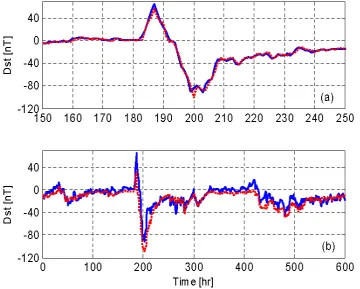
Figures 4(a) presents one-step-ahead (OSA) predictions, over a typical storm period, and the value of MSE for OSA predictions was calculated to be 9.6768. Figure 4(b) presents the long-term predictions (model predicted outputs, MPO). It is clear from Fig. 4 that the identified MSRBF network model provides very good predictions for the Dst index, even during a period of a storm (Dst is near to or less than -100nT).

6. Conclusions

Radial basis function networks possess several attractive properties. Motivated by these attractive properties, a novel hybrid multiscale radial basis function (MSRBF) network has been introduced to model and forecast the Dst index. Compared with traditional single scale (kernel width) RBF networks, the new multiscale (multi-width) RBF network is more flexible and more powerful to describe complex input-output dynamical systems. While the polynomial submodel in the new network can be used to track the linear trend of the underlying dynamical behaviour, the MSRBF submodel can be used to capture the main underlying nonlinear dynamics by employing multiscale basis functions with different centres and widths. This enhances the capability of both the linear models and the traditional radial basis function networks. With a linear-in-the-parameters form, the new network can easily be trained using the forward orthogonal regression (FOR) algorithm, which combines good effectiveness with high efficiency. The identified network model provides very good short term predictions for the Dst index, over the associated data set. Albeit there exists a large discrepancy between long-term predictions and the associated measurements, the model predicts the strong storm very well.

Acknowledgements

References

Baker, D. N., Klimas, A. J., McPherron, R. L., and Buchner, J. The evolution from weak to strong geomagnetic activity: an interpretation in terms of deterministic chaos. Geophys. Res. Lett., 17(1), 41-44, 1990.

Billings, S. A., Chen, S. and Korenberg, M. J. Identification of MIMO non-linear systems suing a forward regression orthogonal estimator. Int. J. Control, 49(6), 2157-2189, 1989.

Billings S. A. and Chen S., The determination of multivariable nonlinear models for dynamic systems using neural networks, in : Neural Network Systems Techniques and Applications, C.T. Leondes, Eds.. San Diego: Academic Press, 231-278, 1998.

Billings, S. A. and Wei, H. L. The wavelet-NARMAX representation: a hybrid model structure combining the polynomial models and multiresolution wavelet decompositions, International

Journal of Systems Science, 36(3), 137-152, 2005a.

Billings S. A. and Wei, H. L. A new class of wavelet networks for nonlinear system identification,

IEEE Trans. Neural Networks, 16(4), 862-874, 2005b.

Boaghe, O.M., Balikhin, M.A., Billings, S.A., and Alleyne, H. Identification of nonlinear processes in the magnetosphere dynamics and forecasting of Dst index, J. Geophys. Res., 106(A12), 30047-30066, 2001.

Burton, R.K., McPherron, R.L. and Russell, C.T. An empirical relationship between interplanetary conditions and Dst. J. Geophys. Res., 80, 4204-4214, 1975.

Chen, S., Billings, S. A., Cowan, C. F. N., and Grant, P. M. Practical identification of NARMAX models using radial basis functions. Int. J. Control, 52(6), 1327-1350, 1990.

Chen, S., Billings, S. A., Neural networks for nonlinear dynamic system modelling and identification,

Int. J. Control, 56(2), 319-346, 1992.

Duda, R. O., Hart, P. E., and Stork, D. G. Pattern Recognition. (2nd ed.). New York: John Wiley & Sons, 2001.

Efron, B. and Tibshirani, R. J. An Introduction to the Bootstrap. New York: Chapman & Hall, 1993.

Goertz, C.K., Shan, L.H., and Smith, R.A. Prediction of geomagnetic activity. J. Geophys. Res., 98(A5), 7673-7684, 1993.

Harris, C. J., Hong, X., and Gan, Q. Adaptive Modelling, Estimation and Fusion from Data : A

Neurofuzzy Approach, Berlin : Springer-Verlag, 2002.

Hartman, E. J., Keeler, J. D., and Kowalski, J. M. Layered neural networks with Gaussian hidden units as universal approximations. Neural Computation, 2(2), 210-215, 1990.

Hernandez, J.V., Tajima, T., and Horton, W. Neural net forecasting for geomagnetic activity.

Geophys. Res. Lett., 20(23), 2707-2710, 1993.

Klimas, A.J., Vassiliadis, D., Baker, D.N. Dst index prediction using data-derived analogues of the magnetospheric dynamics. J. Geophys. Res., 103(A9), 20435-20447, 1998.

Krzanowski, W. J. and Lai, Y. T. A criterion for determining the number of groups in a data set using sum-of-squares clustering. Biometrics, 44(1), pp. 23-34, 1988.

Leontaritis, I. J. and Billings, S. A. Input-output parametric models for non-linear systems, Int. J.

Control, 41(2), 303-344, 1985.

Liu, G. P. Nonlinear Identification and Control : A Neural Network Approach. London : Springer, 2001.

Lundstedt, H., Gleisner, H., Wintoft, P. Operational forecasts of the geomagnetic Dst index. Geophys.

Res. Lett., 29(24), Art. No. 2181, 2002.

McPherron, R.L. Predicting the Ap index from past behaviour and solar wind velocity. Physics and

Chemistry of the Earth Part C, 24(1-3), 45-56, 1999.

O’Brien, T.P. and McPherron, R.L. An empirical phase space analysis of ring current dynamics: solar wind control of injection and decay. J. Geophys. Res.,105 (A4), 7707-7719, 2000.

Park, J. and Sandberg, I. W. Universal approximation using radial-basis-function networks. Neural

Computation, 3(2), 246-257, 1991.

1990.

Pulkkinen, T.I. and Baker, D.N. Global substorm cycle: what can the models tell us? Surveys in

Geophysics, 18, 1-37, 1997.

Schwarz, G. Estimating the dimension of a model, The Annals of Statistics, 6, 461-464, 1978.

Sharifi, J., Araabi, B. N., Lucas, C. Multi-step prediction of Dst index using singular spectrum analysis and locally linear neurofuzzy modelling. Earth Planets and Space, 58 (3), 331-341, 2006.

Takalo, J., and Timonen, J. Neural network prediction of AE data. Geophys. Res. Lett., 24(19), 2403-2406, 1993.

Vassiliadis, D., Klimas, A.J., Baker, D.N., and Roberts, D.A. A description of the solar-wind magnetosphere coupling based on nonlinear filters. J. Geophys. Res.,100(A3), 3495-3512, 1995. Vassiliadis, D., Klimas, A.J., Valdivia, J.A., and Baker, D.N. Models of Dst geomagnetic activity and

of its coupling to solar wind parameters. Physics and Chemistry of the Earth Part C, 24(1-3), 107- 112, 1995.

Watanabe, S., Sagawa, E., Ohtaka, K., and Shimazu, H. Prediction of the Dst index from solar wind parameters by a neural network method. Earth Planets and Space, 54 (12), 1263-1275, 2002. Wei, H.L., Billings, S.A. and Balikhin, M.A. Prediction of the Dst index using multiresolution wavelet

Models. J. Geophys. Res., 109(A7), A07212, doi:10.1029/2003JA010332, 2004a.

Wei, H. L., Billings, S. A., and Liu, J. Term and variable selection for nonlinear system identification,

Int. J. Control, 77(1), 86-110, 2004b.

Wei, H. L., Billings, S. A., and Balikhin, M. A. Wavelet based nonparametric NARX models for nonlinear input-output system identification. Accepted by International Journal of Systems

Science, 2006.

Wu, J.G., and Lundsted, H. Neural network modelling of solar wind magnetosphere interaction. J.