S. Zandi
Geoinformatics Research Centre, Auckland University of Technology, Auckland, New Zealand , A. Ghobakhlou and P. Sallis
Email:
Abstract: Soil pH has a major effect on plant nutrient availability by controlling the chemical structure of the nutrient. Adjusting soil acidity or alkalinity improves soil nutrition without adding extra fertilizers. Soil nutrients needed by plants in the largest amount are referred to as macronutrients. In addition to macronutrients, plants also need trace nutrients and both macro and trace nutrient availability is controlled by soil pH. Understanding of spatial variability of soil properties is important in site-specific management. Analysis of spatial variation of soil properties is fundamental to sustainable agricultural and rural development. The special variability of soil property is often measured using various interpolation methods resulting in map generation. Selecting a proper spatial interpolation method is crucial in surface analysis, since different methods of interpolation can lead to different surface results. Among statistical methods, geo-statistical kriging-based techniques have been frequently used for spatial analysis and surface mapping.
In this work, three common interpolation methods are used to study the spatial distributions of soil pH in a vineyard. Interpolation techniques were used to estimate the pH measurement in unsampled points and create a continuous dataset that could be represented over a map of the entire study area. The method investigated includes; Inverse Distance Weighting (IDW), Radial base Function (RBF) and Ordinary Kriging (OK). The performance of conventional statistics showed that soil pH had a law variation in this study.
Experimental anisotropic semivariograms were fitted with the Spherical, Exponential, Gaussian and Exponential models and the Exponential model was found as the best fitted model using the cross-validation method. The performances of interpolation methods were evaluated and compared using the cross-validation. The results showed that RBF method performed better than IDW and OK for prediction of the spatial distribution of topsoil pH (Figure 1).
Figure 1: Prediction map of soil pH generated by: (a) IDW; (b) RBF and (c) OK
Keywords: Geostatistics, Spatial Interpolation, Ordinary Kriging (OK), Inverse Distance Weighting (IDW), Radial Base Function(RBF), Surface mappingIntroduction
1. INTRODUCTION
For an agricultural system to be sustainable it must be soil restorative that is the productivity, quality and capacity of soil must be preserved and improved (Rattan, 1995). Managing spatial variability which is popularly known as precision farming is essential for serving dual purpose of enhancing productivity and reducing ecological degradation. The focus of precision farming is to optimize the crop production and reduce soil fertility losses. The first step in Site-specific management is measuring the spatial variability of soil property using map generation. In order to determine the spatial variability of soil properties the best method needs to be identified. The variety of available interpolation methods has led to questions about which is most appropriate in different contexts and has stimulated several comparative studies of relative accuracy (Zimmerman et al., 1999). There is no single preferred method for data interpolation. Among statistical methods, geo-statistical kriging-based techniques have been often used for spatial analysis (Deutsch, 2002). Inverse Distance Weighting (IDW) and its modifications are the most often applied deterministic interpolation method (Nalder and Wein, 1998). Ordinary Kriging (OK), Inverse Distance Weighting (IDW), and Radial Basis Functions (RBF) are three well-known spatial interpolation techniques commonly used for characterizing the spatial variability and interpolating between sampled points and generating the prediction maps.
The main objective of this study is to review and evaluate the three common interpolation methods namely; Ordinary Kriging (OK), Inverse Distance Weighting (IDW), Radial Base Function (RBF) and generate maps of soil pH property using these methods. The accuracy and efficiency of the generated maps are also examined and the most fitting technique for the soil pH in the study area is identified.
2. MATERIALS AND METHODS
2.1. Study Area and Data
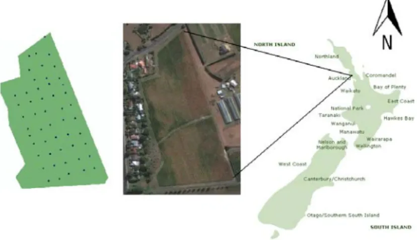
The data were collected from the Kumeu vineyard located in Kumeu region in Auckland, New Zealand in May 2011 (Figure 2). Fifty four soil samples were collected as part of an ongoing research project in the Geoinformatics Research Centre (Scannavino et al., 2011). The size of the study area was approximately 400 x 150 m. Soil samples were collected from three depths: 5-25cm, 25-45cm and 45-55cm. Soil pH was measured three times on the field using Field Scout pH 110 Meter data logger. Soil moisture and temperature were collected along with the geo-coordination for each sampling point. In this study we only examine the pH reading from the topsoil (5-25cm).
Figure 2: Location of study area and sampling patterns 2.2. Methods
Statistical analyses were performed in three stages. First, the frequency distributions of data were analyzed and normality was tested using the Anderson Darling normality test. The Anderson-Darling test is used to test if a sample of data came from a population with a specific distribution. It is a modification of the Kolmogorov-Smirnov (K-S) test and gives more weight to the tails than does the K-S test. The K-S test is distribution free in the sense that the critical values do not depend on the specific distribution being tested. The Anderson-Darling test makes use of the specific distribution in calculating critical values. This has the
advantage of allowing a more sensitive test and the disadvantage that critical values must be calculated for each distribution (nist, 2010). Secondly, the distribution of data was described using conventional statistics such as mean, maximum, minimum, median, Standard Deviation (S.D), Coefficient of Variation (CV), and skewness. These analyses were conducted using the Minitab software package. Thirdly; Global trend analysis was preformed to examine the existence of trend in pH data. Global trend is a dominant process that affects the measurement deterministically. A three-dimensional perspective of the data was created using the trend analysis tool of ArcMap 9.2 software package. Global trend exists if definite polynomial pattern can fit through the data.
Deterministic interpolation techniques create surfaces from measured points, based on either the extent of similarity (Inverse Distance Weighted) or the degree of smoothing (Radial Basis Functions). Geostatistical interpolation techniques use the statistical properties of the observed points. Geostatistical techniques quantify the spatial autocorrelation among measured points and account for the spatial configuration of the sample points around the prediction location (Esri, 2008). The following briefly describes the above mentioned methods:
Inverse Distance Weighting (IDW): All interpolation methods have been developed based on assumption that nearby points have more correlations and similarities than distant observations. In IDW method, it is assumed that the rate of correlations and similarities between neighbors is proportional to the distance between them that can be defined as a distance reverse function of every point from neighboring points (Saffari, Yasrebi, Sarikhani, & Gazni, 2009). IDW method works best with evenly distributed points. The main factor affecting the accuracy of inverse distance interpolator is the value of the power parameter ‘p’ (Isaak and Srivastava, 1989). The size of the neighborhood and the number of neighbors are also relevant to the accuracy of the results.
Ordinary Kriging (OK): This method provides an estimate at an unsampled point based on the weighted average of observed neighboring points within a given area. Unlike IDW, kriging method is not deterministic but extends the proximity weighting approach of IDW to incorporate random components where the exact point is unknown. The weights in the kriging method are based on the distance between the measured points and the prediction points and the overall spatial arrangement of the measured points (Lou, Taylor, & Parker). OK is one of the most basic of kriging methods. The spatial autocorrelation between measured sample points was examined using the semivariogram /covariance cloud. Experimental anisotropy semivariogram were examined to model the spatial relationship in the dataset and to find out the best fit model that passes through the points in the semivariogram. The weights in OK depend on a fitted model to the measured points, the distance to the prediction location, and the spatial relationships among the measured values around the prediction point. Kriging methods use the semivariance to estimate the spatial and statistical relationships and then perform the interpolation and calculate the surface.
Radial Basis Function (RBF)
2.3. Comparison and Evaluation Procedures
: Radial Base Function methods are considered as exact interpolation techniques. The exact interpolators predict values identical with those measured at the same point and the generated surface requires passing through each measured points. The predicted values can vary above the maximum or below the minimum of the measured values (Nikolova and Vassilev, 2006). There are five different basis functions: thin- plate spline, spline with tension, completely regularised spline, multi-quadratic function and inverse multi-multi-quadratic function. There is a small difference between basis functions and the generated surfaces are slightly different (Karydas et al., 2009). The estimated values of the methods are based on a mathematical function that minimises total curvature of the surface, generating quite smooth surfaces. The smoothness of the resulting surface is controlled by a smoothing parameter.
In this study, Spherical, Exponential and Gaussian functions were examined to determine the best model to fit semivariogram that is used in OK interpolation method. A cross-validation was used to find the best model. The performance of each interpolation technique, in terms of the accuracy of predictions, was assessed by comparing the deviation of estimates from the measured data by performing a cross-validation technique over the entire dataset. In a cross validation procedure each data point is removed from the data set, one at a time, and predicted value is return by performing interpolation algorithm on the rest of dataset. This yield a list of estimated values of variable data paired to the test data. The comparison of performance between interpolation techniques was achieved by using the Mean Error (ME) and Root Mean Square Error (RMSE).
3. EXPERIMENTS AND RESULTS
Conventional statistics were performed on available dataset and the summary statistic is shown in Table 1. In this study, soil pH had Coefficient Variation (CV) of 7.24%. According to the variability of soil properties guidelines provided by Warrick (1998) there was a law variation (CV <15%) of soil pH in this study area.
Table 1: Descriptive statistics for soil pH
Mean SE
Mean
Standard Deviation
Variance CV (%) Median Min Max
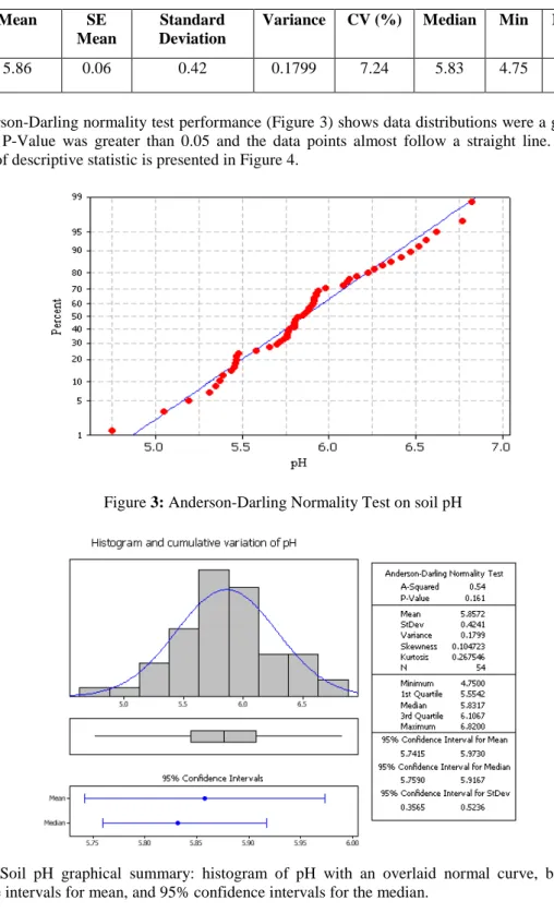
5.86 0.06 0.42 0.1799 7.24 5.83 4.75 6.82
The Anderson-Darling normality test performance (Figure 3) shows data distributions were a good fit. The calculated P-Value was greater than 0.05 and the data points almost follow a straight line. A graphical summary of descriptive statistic is presented in Figure 4.
Figure 3: Anderson-Darling Normality Test on soil pH
Figure 4: Soil pH graphical summary: histogram of pH with an overlaid normal curve, boxplot, 95% confidence intervals for mean, and 95% confidence intervals for the median.
Trend analysis showed that there was no significant global trend for the soil pH in this area (Figure 5). More specifically, both North-South and East-West trend lines did not exhibit an obvious curve. The reason
that the North-South projection was not perfectly flat can be attributed to the geographic characteristics of the study area which has a very gentle slop.
Figure 5: Trends of soil pH
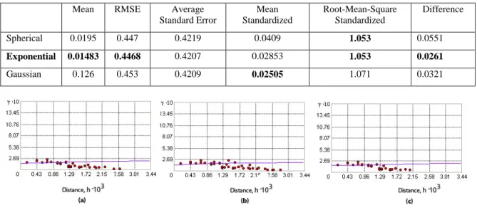
In order to identify the possible spatial structure of the soil pH, experimental anisotropic semivariograms were calculated. The Exponential function was identified as the best fitted model using cross- validation. The result of cross-validation is provided in Table 2. The best model was selected based on four criteria: the standardized mean nearest zero, the smallest Root-Mean-Squared prediction Error (RMSE), the average standard error nearest the root-mean-squared prediction error and the standardized root-mean-squared prediction error nearest one. In this study, the Exponential model meets the most of the requirements for the best fitted model. Figure 6 shows the experimental semivariograms generated by Spherical, Exponential and Gaussian models.
Table 2: Cross Validation Result
Mean RMSE Average
Standard Error Mean Standardized Root-Mean-Square Standardized Difference Spherical 0.0195 0.447 0.4219 0.0409 1.053 0.0551 Exponential 0.01483 0.4468 0.4207 0.02853 1.053 0.0261 Gaussian 0.126 0.453 0.4209 0.02505 1.071 0.0321
Figure 6: Experimentalsemivariograms: (a) Spherical; (b) Exponential and (c) Gaussian
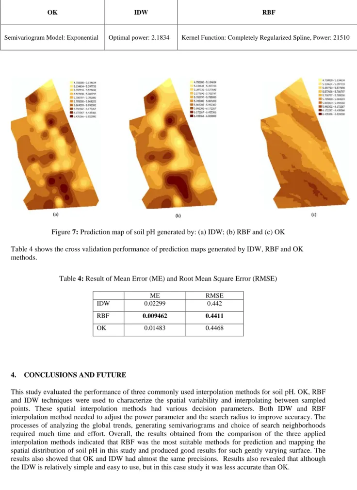
The interpolation methods were implemented to estimate unmeasured data values and create surfaces from measured points. The parameters used in interpolation methods for creating the prediction maps of soil pH are presented in Table 3. The mapping result of IDW, RBF and OK are shown in Figure 7.
Table 3: Parameters of interpolation methods used for prediction maps of soil pH (searching neighborhood of 15)
OK IDW RBF
Semivariogram Model: Exponential Optimal power: 2.1834 Kernel Function: Completely Regularized Spline, Power: 21510
Figure 7: Prediction map of soil pH generated by: (a) IDW; (b) RBF and (c) OK Table 4 shows the cross validation performance of prediction maps generated by IDW, RBF and OK methods.
Table 4: Result of Mean Error (ME) and Root Mean Square Error (RMSE)
ME RMSE
IDW 0.02299 0.442
RBF 0.009462 0.4411
OK 0.01483 0.4468
4. CONCLUSIONS AND FUTURE
This study evaluated the performance of three commonly used interpolation methods for soil pH. OK, RBF and IDW techniques were used to characterize the spatial variability and interpolating between sampled points. These spatial interpolation methods had various decision parameters. Both IDW and RBF interpolation method needed to adjust the power parameter and the search radius to improve accuracy. The processes of analyzing the global trends, generating semivariograms and choice of search neighborhoods required much time and effort. Overall, the results obtained from the comparison of the three applied interpolation methods indicated that RBF was the most suitable methods for prediction and mapping the spatial distribution of soil pH in this study and produced good results for such gently varying surface. The results also showed that OK and IDW had almost the same precisions. Results also revealed that although the IDW is relatively simple and easy to use, but in this case study it was less accurate than OK.
It is reasonable to conduct further experiments on soil pH obtained from two other depths in order to validate the results from this study. It is desirable to compare these results with soil pH measured in laboratory.
5. REFERENCES
Esri. (2008). Deterministic methods for spatial interpolation. Retrieved August 12, 2011, from esri: http://help.arcgis.com/en/arcgisdesktop/10.0/help/index.html#//003100000023000000.htm
Deutsch, CV.(2002) Geostatistical reservoir modeling, 1st edn. Oxford University Press, New York Isaaks, E. H. and R. M. Srivastava. (1989). An Introduction to Applied Geostatistics. Oxford Univ. Press,
New York, Oxford.
Karydas, C.G., Gitas, I.Z., Koutsogiannaki, E., Lydakis-Simantiris, N., Silleos, G.N. (2009). Evaluation of spatial interpolation techniques for mapping agricultural topsoil properties in Crete. EARSeL eProc. 8, 26–39.
Lou, W., Taylor, M., & Parker, s. (n.d.). Spatial interpolation for wind data in England and Wales. Retrieved 08 10, 2011, from InterMet: http://intermet.csl.gov.uk/wind.pdf
Nalder, I.A.; Wein, R.W. (1998). Spatial interpolation of climatic normals: Test of a new methods in the Canadian boreal forest. Agricultural and Forest Meteorology. 92: 211-225.
Nikolova N, Vassilev S. (2006). Mapping precipitation variability using different interpolation methods. Proceedings of the Conference on Water Observation and Information System for Decision Support (BALWOIS).s May 2006,Ohrid, Macedonia, 25-29.
nist. (2010). Retrieved August 11, 2011, from NIST/SEMATECH e-Handbook of Statistical Methods: http://www.itl.nist.gov/div898/handbook/eda/section3/eda35e.htm
Rattan, L.(1995). Sustainable management of soil resources in the humid tropics, UN University, New York, Paris.
Saffari, M., Yasrebi, F., Sarikhani, R., & Gazni, M. (2009). Evaluation and Comparison of Ordinary Kriging and Inverse Distance Weighting Methods for Prediction of Spatial Variability of Some Soil Chemical Parameters. Research Journal of biological Sciences. , 4.
Scannavino Jr. F., Ghobakhlou, A., Perez-Kuroki, A., and Sallis, P., and Cruvinel P. (2011). Spatial variability of soil pH: a case study in vineyards. In proceedings of IEEE workshop on Instrumentation and Measurement Society New Zealand Chapter Workshop on Smart Sensors, Measurement and instrumentation (abstract), Auckland University of Technology (AUT), New Zealand, 10-11 March 2011. p 24.
Warrick, A.W. (1998). Spatial Variability In Environmental Soil Physics, Hillel, D. (Ed.). Academic Press, USA., pp: 655-675.
Zimmerman, D., Pavlik, C., Ruggles, A. and Armstrong, M. P. (1999). An experimental comparison of ordinary and universal Kriging and inverse distance weighting. Mathematical Geology, 31 (4).