Munich Personal RePEc Archive
Demographic changes and economic
development: Application of the vector
error correction model (VECM) to the
case of Ethiopia
Wako, Hassen
Jimma University
October 2012
1
Journal of Economics and International Finance Vol. 4(10), pp. 236-251, October, 2012 Available online at http://www.academicjournals.org/JEIF DOI: 10.5897/JEIF12.039 ISSN 2006-9812 ©2012 Academic Journals
Full Length Research Paper
Author’s Final (Pre-publication) Version
Demographic Changes and Economic Development: Application of
the Vector Error Correction Model (VECM) to the Case of Ethiopia
Hassen Abda Wako
Department of Economics, College of Business and Economics, Jimma University,
Jimma, Ethiopia Tel: +251911083176 Email: [email protected]; [email protected]
ABSTRACT
Ethiopia is one of the countries with high fertility, rapidly growing and largely young population. At the same time, it is among countries with weak and poorly focused population policy. In light of this, this study intended to assess the causation between demographic factors and economic development in Ethiopia. To this end, it applied vector-error-correction model (VECM) to data on economic, demographic and other variables obtained from secondary sources, accompanied by descriptive analysis of the relationship of population with HDI, agricultural landholdings and forestland. VECM results indicated robust and negative long run relationship between per capita income
and population growth and a positive one between the former and growth of workers –
with bidirectional causality in both cases. That is, rises in per capita income reduce the growth of (dependent) population and enhance that of workers, and vice versa. Conversely, slower growth of population or faster growth of workers raises per capita income. Short run relationships turned out to be weak and non-robust to alternative model specifications. The descriptive analysis signified inverse associations of population growth with landholding, forest coverage and HDI score. These findings point to a need for meaningful efforts to incorporate population matters into the policy arena. ______________________________________________________________________
2
INTRODUCTION
The debate on the relationship between population and development has a long history. As Panayotou (2000) discusses in some detail, contrasting views on the issue go back to the time of Plato and Aristotle. The same source points out that even in its modern version, the debate had existed some years before the very influential 1798 book of Thomas Malthus. According to Todaro and Smith (2006), the very aged debate on population-development relationship is yet to continue into the future.
Since Malthus‟ 1798 book on population, many scholars have considered the imbalance between population and resources in general, and the implications of this imbalance in particular, as a serious matter. In words of Singh and Singh (1997: 4), for instance,
“host of social evils, famines and wars, perpetuation of vicious circle of poverty and
accordant problems are [more] often than not ascribed to inequilibrium in
population-resource situation.” However, this view is far from indisputable as there are many
scholars on the other extreme – population optimists – who believe that “it will always
be possible for the world to absorb more people and reap the economic benefits of a
larger labor force” Latimer and Kulkarni (2008).
Empirically, studies have failed to suggest an overall dominance of one view over the other. The majority of studies on population-development relationship in the 1950s and 1960s claimed a negative relationship between the two variables with causality running from population to development. While these studies had population-alarmist conclusions, they differed from early Malthusian position mainly in treating population growth as an exogenous variable. By treating population growth as an exogenously determined variable, classical economists attributed the negative effect of population growth on per capita income to the idea that larger population dilutes the amount of physical capital coupled with diminishing marginal returns (Birdsall, 1988; Ehrlich and Lui, 1997). Extending such analysis of economic growth through including the role of human capital (in line with the endogenous growth theories), Mankiw et al. (1992) have also found that population growth negatively affects growth in GDP per capita.
In the late 1970s and during the 1980s, researches began to become less assertive of the negative impact of population on development and started to come up with
conclusions resembling: controlling population growth is likely to help developing
3
have described the major problem of this world to reside not in population but in lack of favorable economic policies and good governance, corruption, and unjust distribution of resources and opportunities (Merrick, 2002; Todaro and Smith, 2006). The revisionist conclusions of the studies in the 1980s may not have come about on themselves, but by the keen arguments of and some empirical supports for the optimist view since 1980s (Keskinen, 2008).
In general, empirical results regarding population-development debate are mixed. As a remark to the discussion of contrasting findings, Nafziger (2006) has forwarded
“Population growth is likely to hamper growth in the first few decades of the 21st century
in Africa and parts of South Asia unless economic, population, and environmental
policies change.” (Nafziger, 2006: 296).
The cause-effect relationship between population and development is not the same across the board. Based on the cases of twenty countries, Darrat and Yousif (1999) have found evidences of causality running from population to economic development, from economic development to population, and in both directions. While population has positively affected economic development in more than half of the countries in their study, population growth is the effect of economic development for poor countries. Countries at low level of development are likely to experience higher population growth, and this relationship will tend to vanish and finally disappear as they progress.
The situation in most developing countries, especially those in Sub-Saharan Africa, looks less controversial. Even for scholars who hold that population could have either positive or negative effects on the economy, this region provides a point in case for the negative effect of population on economic development. For those who emphasize positive effects of demographic variables, sub-Saharan Africa is a region characterized by factors likely to undermine such benefits. In relation to the economic benefits of
falling fertility and mortality rates and rising share of working-age population – the
demographic dividend – Bloom et al. (2007) have shown that sub-Saharan Africa has
the same chance of enjoying this benefit as the rest of the world. However, reaping this
benefit is conditional on institutional quality and “… the average institutional quality in
Africa lags significantly behind the average in ROW [the rest of the world]” (Bloom et al.,
2007:20). Despite the equal potential that sub-Saharan Africa has with the rest of the
world, it is still the case that “While most regions around the world are evolving through
the demographic transition Africa stands as an outlier” (Bloom et al., 2007:2).
4
The place of population issues in the Millennium Development Goals (MDGs) presents a point in case. Yousif (2009) presents how the MDGs have played down the importance of demographic factors in development efforts. Praising the role of MDGs in mobilizing forces for poverty reduction, Fisher and Newman (2011) are also among
those who criticize the neglect of population – “the missing link” – by these goals. A
question that logically follows from here is then: Why the neglect to population issues?
An answer to the above question may perhaps reside in the view of international policy makers on the population-development debate. Accompanying such a suspicion is the changing position of the United Nations Population Fund (UNFPA) on the issue over time. In early days, UNFPA identifies itself with population-pessimism and Malthusian-based recommendations of birth control through family planning. Overtime, this organization has shifted to recommending rights-based access to birth control and the significant role of empowering women and educating girls in controlling population size. While it still argues in favor of slower population growth, it has been shifting away from its presumption that causality runs from population to economic development. In its 2011 report, UNFPA has forwarded some recommendations that clearly show its shift towards considering development as cause and population change as effect. The first
recommendation on a summarizing page of this report, headed Seven Opportunities for
a World of 7 Billion, reads: “Reducing poverty and inequality can slow population
growth.” Similarly, the fourth point forwarded reads: “Ensuring that every child is wanted
and every childbirth safe can lead to smaller and stronger families” (UNFPA, 2011).
The Ethiopian case seems to mirror this changing global view on population-development debate. For instance, the neglect of population growth as a policy issue is common to most (if not all) reports of the Ministry of Finance and Economic Development (MoFED). Even in the limited number of lines devoted to population issue,
these reports put it in a subsidiary position. In one of such reports, MoFED (2006) –
after detailing the manifestations of the multi-dimensional successes of the country –
gives the credit of leading developmental concerns to labor and land productivity. The report acknowledges the issue of rapidly growing population as an additional challenge.
5
and 2000, the pace of decline dropped off subsequently. The total fertility rate declined only from 5.5 in 2000 to 5.4 in 2005. This slow down in reducing total fertility rate was primarily because of little change in rural fertility (Macro International Inc., 2007).
The general shift in the view of policymakers on the population-development debate may have some concrete theoretical and empirical foundations. For Ethiopia (a country listed among the top countries with concerns of high fertility rates), however, it demands firm evidence to push population issues to the periphery. The fact is that no such evidence justifying the neglect of population growth in policy arena exists. Even with the
remarkable attention the country is apparently paying to “statistical success” (as a tool
for convincing others of our “sustained development”), quantitative data and references
to empirical researches on population-development link hardly appear in governmental reports and policy papers. While statistics (or numbers) have undoubtedly played a
significant role in our “development achievements”, our neglect of population matters
has not benefitted from “statistical successes”. Nor do we have meaningful efforts made
to deal with the demographic challenges of the country. Ethiopia has never revisited its population policy since the one written in 1993. Ringheim et al. (2009) have pointed out this weakness while discussing the window of opportunities the country could enjoy.
Given the remarkable contrast between the demographic situation and the importance attached to population matters in policymaking, this study pursued the general objective of assessing the causal relationship between population and economic development in Ethiopia. Specifically, it tried to evaluate the direction and strength of the link between the growth of population and its components on one side and GDP per capita on the other. Besides, it attempted to assess the association between population growth and human development index (HDI) and highlight the pressure of population growth on agricultural land and forest coverage of the country. The study generally covered the period from 1950 to 2011. However, availability of data on some variables limited the coverage of some sections and/or sub-sections to shorter time spans.
MATERIALS AND METHODS
Types and Sources of Data
6
Population of the United Nations Population Fund (UNFPA); Penn World Tables of Heston et al. (2011).
Model Specification
The logical starting point for evaluating the cause-effect relationship between population and economic performance lies in establishing a theoretical link between the two. In this regard, the common practice is to employ the growth rate (or size) of total population for the former and the growth rate (or size) of GDP per capita for the later. Using size or growth rate of total population, however, ignores the heterogeneity within the population in terms of age (dependants versus independents) and economic activity (those in the labor force as employed or unemployed versus those economically inactive) among others. Two hypothetical countries identical in all aspects (including population size), except that one has more of its population in the labor force and lower rate of unemployment than the other does, are not expected to show the same relationship between demographic and economic variables. Dissatisfaction with the use of a single
measure of demographic factors – size or growth rate of total population – has led to the
examination of various aspects of the demographic side of the equation. Bloom et al. (2001), Yousif (2009), Prettner and Prskawetz (2010) are among works calling attention to the need for and the significance of such a shift.
Consequently, disaggregating the effect of population growth into the effects of
population (size or growth rate) in various age groups – most notably into dependent
and working-age populations – emerged. Besides, considering birth rates and death
rates separately instead of population growth rate has also joined the literature in the area. Kelley and Schmidt (1995) is one of the works forerunning both such practices. They have found significantly differing conclusions on population-development debate arising just from using traditional measures of demography or the disaggregated ones.
In line with these arguments, this study experimented with the inclusion of the size and growth rate of total population, of workers (or employment), and of dependents. As a starting point, it assessed the relationship between each of these three demographic variables on the one hand and real GDP per capita on the other in the setting of bivariate analysis. Lack of sufficient data on birth and death rates did not permit separate treatment of these variables.
7
(gross capital formation), exports, imports, foreign direct investment and foreign aid. Given the small size of the time series data available relative to the requirement of the estimation techniques (specified after a while), the number of variables should be restricted. Accordingly, the choice of covariates in the regression equations depended on the length of the time span for which data are available. For instance, the variables fiscal deficit, foreign direct investment, foreign aid and depreciation of capital did not join the analysis on grounds of data availability. Besides, the variables imports, dependency ratio and population density were dropped after tests of stationary proved them to be of different order of integration. Moreover, the statistical performance of the estimates from VAR and VEC models has been well-studied and well-established for models with a few number of variables (Moneta et al., 2011).
Hence, the estimation of and tests about the relationship between demographic and economic variables involved the following six variables:
RGDPPC = Real GDP per capita (as a measure of economic performance);
POPGR = population growth rate (change in natural logarithm of population size); EMPLGR = growth rate of total employment (change in ln(number of workers)); OPEN = Openness (measured by the sum of exports and imports over GDP);
HUMAN = Human capital (government‟s health and education expenditure
consumed by households);
INVEST = Domestic Investment (gross capital formation);
All these variables, measured at constant 2005 International Dollars (using chain series) are from Heston et al. (2011). Two of these variables are growth rates while the remaining four are in their levels (or log-levels). The order of integration of these variables assisted the choice between their levels (or log-levels) and growth rates.
Besides, models with regime dummies (1950 – 1973, 1974 – 1991, 1992 – 2009) were
estimated.
Methods of Data Analysis
This study relied on both descriptive statistics and econometric techniques. Under the descriptive analysis, numbers showing absolute sizes and changes, percentages,
ratios, and growth rates – summarized in tables and graphs – were used to show the
relationship between various measures of economic performance and measures of population dynamics.
8
(and establish the direction of causality for) short-run relationships among stationary (or I(0)) variables and co-integrating (long-run) relationships among difference-stationary (or I(1)) variables. Accordingly, the following set of regression equations was estimated:
i p t p 2 t 2 1 t 1 1 t
t α.ECT ΓΔY Γ ΔY ... Γ ΔY ε
ΔY
where: ΔYt
RGDPPCt POPGRt EMPLGRt OPENt HUMANt INVESTt
Γi s (i = 1, 2, …, p) are matrices of short run parameters;α is a matrix of adjustment parameters (reflecting dynamics towards equilibrium);
1 t 1 t βY
ECT is a matrix of error correction terms (with β a matrix of long-run
parameters capturing co-integrating relationships among variables);
t = time period (that is, year taking values 1, 2, 3 …);
∆ = difference (for example, ∆RGDPPCt = RGDPPCt– RGDPPCt-1); and
i = lag running from 1 (one year back) up to p (the maximum lag); respectively.
Moreover, dummy variables for regimes (Derg = 1 between 1974 and 1991 and = 0 elsewhere; EPRDF = 0 before 1992 and =1 then after) were included into the regression equation.
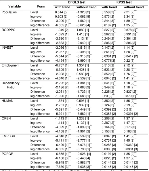
As VEC models demand the order of integration of the variables, the first task was testing for the stationarity of the variables. Two tests of unit-root/stationarity served this purpose: the Generalized-Least-Squares transformed Augmented Dickey-Fuller (DFGLS) test, and the Kwiatkowski-Phillips-Schmidt-Shin (KPSS) test. The DFGLS test was preferred to the commonly used Augmented Dickey-Fuller (ADF) test as the former accounts for the presence of heteroskedasticity and autocorrelation. The DFGLS test also performs better that the Phillips-Perron (PP) test, another test which accounts for the presence of heteroskedasticity and autocorrelation (StataCorp, 2009). The study used the KPSS test to complement the DFGLS test; the order of integration of a variable was inferred from the agreement of the conclusions of the two tests. Such a role for the KPSS test to complement other tests (as the DFGLS test here) was established on the ground that this test has the null hypothesis of stationary series as opposed to others with the null of unit root in the series (Baum, 2000).
Where the two tests – DFGLS and KPSS – happened to choose different lag lengths,
9
To test for stationarity and to estimate VEC models, this study has used Schwarz‟s
Bayesian Information Criterion (SBIC), Hannan and Quinn Information Criterion (HQIC),
Akaike‟s Information Criterion (AIC), and Final Prediction Error (FPE) for determining
the optimal lag. In cases of disagreement among these criteria, the lag length preferred
by each criterion was checked. In testing for the rank of co-integration, Johansen‟s
likelihood ratio (LR) test – using both trace and maximum statistics – was employed,
supplemented by the usual SBIC and HQIC. When two/ more models (differing by trend specification or lag length) passed all pre-estimation tests, post-estimations tests (VECM-stability, autocorrelation in error terms, and stationarity of the co-integrating equation) assisted for discriminating between/among the qualifying models.
The statistical package used to handle most of the tests and estimations is Stata (version 11.0). The components of Stata necessary for undertaking the KPSS test of stationarity that are not part of the official Stata 11.0 version, authored by Christopher F. Baum, were downloaded from the website of the Stata-community. The tests and estimations of models involving dummy variables were conducted with the help of JMulTi (version 4.23).
RESULTS AND DISCUSSION
This section deals with the presentation and analyses of data on the trend and components of population dynamics, and its relationship with measures of economic performance, namely, trends of HDI, changes in arable land, forest coverage and agricultural landholdings, and real GDP per capita.
Trend and Components of Population Dynamics
As World Bank (2010) data depict, with a total population of around 22.6 million in 1960, Ethiopia experienced a population blast that resulted in more than 82.8 million people
by 2009. Indeed, the population size doubled between 1985 and 2009 – signifying a
10
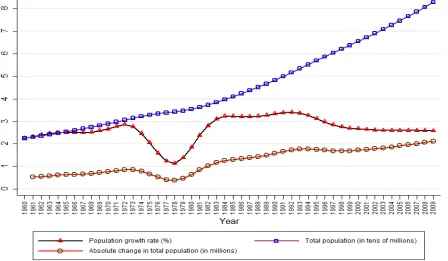
Figure 1: Size, growth rate and absolute change in size of total population: 1960 – 2009
Source: Constructed Based on Data from World Bank (2010)
Figure 2: Population growth rate and the rate of natural increase: 1960 – 2009
11
Though the total population size was increasing over time (and is likely to do so for
some decades to come), it seemed that the rate at which population size rises has
currently stabilized at about 2.6 percent per annum (UN, 2011a). However, there is no
consensus among different sources on this story of population growth rate stabilizing
around 2.6%. The data from Heston et al. (2011) indicated the rate of population growth
to be 3.2 percent in 2009; it shared the stabilizing story of the UN though.
While this slow down in the speed of population dynamics could be encouraging, it is far from suggesting that Ethiopia overcame the population problem. With so many millions of people already on the ground, more and more millions will subsequently be
welcomed every year – exposing the concern of population momentum. For instance,
while the rate of population growth dropped from about 3.4 percent in 1992 to about 2.58 percent in 2009, the absolute change in population size rose from about 1.73 million extra people in 1992 to about 2.11 million extra people in 2009 (Figure 1).
The particular pattern taken by variables in Figure 1 hinges on the rate of natural increase (i.e., the difference between birth rate and death rate) and the rate of net migration (the difference between immigration and emigration rates). Perhaps due to its relatively smaller contribution to population growth, and poor and discontinuous data, international migration usually takes a subsidiary position in discussions of population dynamics. In fact, the comparison between the rate of population growth and the rate of natural increase revealed that the two rates generally behave similarly (Figure 2).
However, this could not justify the ignorance of migration in analyzing population dynamics. For instance, the deep valley in population growth rate in the 1970s was neither because of a sudden drop in birth rate nor due to a sudden climb in death rate. The crude birth rate and the crude death rate (more importantly the difference between them) were generally stable. Thus, the divergence between the two rates shown in Figure 2 is indicative of the role international migration played in explaining population dynamics. Though year-by-year data are not available on international migration, the five-year average data on net immigration from UN (2011a) gives a picture very consistent with the divergence between the two series in Figure 2.
Political instability associated with the 1974 revolution was perhaps the most apparent phenomenon that explains the unusually important place of international migration. The radical shift in ideology of the government from Western-oriented feudalism to socialism
and the subsequent „Nech Shibir‟ – „Qey Shibir‟ (to mean White Terror – Red Terror)
12
number of emigrants. The subsequent reversal in the net migration (during 1980–1985)
was possibly due to emigrants returning home after relative stability came to the country as Mengistu Hailemariam effectively eliminated all his political opponents. The return of negative net immigration in the 1990s was also likely to be the result of political insatiability following the change of regime in 1991.
Even if international migration has had a significant influence, the components of natural
increase – fertility and mortality – were by far the main actors in population dynamics of
the country. World Bank (2010) data indicate the following. For the period from 1960 to 2008, the crude birth and death rates of the country averaged 45.72 births and 18.68 deaths per 1000 people respectively. While this implied an average rate of natural increase equal to 27.04 per 1000 people, the rate of net immigration was relatively
immaterial (averaged – 0.59 per 1000 people between 1960 and 2010).
The crude birth and death rates were above the average rates for sub-Saharan Africa.
For the period 1980–2008, for which data for comparison were available, the crude birth
rate of Ethiopia (44.7 births per 1000 people) was above the average for sub-Saharan Africa (42.9). Similarly, the average crude death rate (16.6) was above the corresponding average for sub-Saharan Africa (15.8). The gap in death rate between Ethiopia and sub-Saharan Africa (and developing countries as a group) was narrower than the gap in birth rates. Thus, while reducing mortality remains a concern of development policy, the relatively high birth rate seems to be of a more critical panic.
Nevertheless, in its World Fertility Policies, UN (2011b) describes Ethiopia as a country with a major government concern about the high level of adolescent fertility but with no policy to reduce it. Contraceptive prevalence rate (for any method) was as low as 15% and unmet need for family planning was as high as 34% (both figures in 2005). This combination suggested that there exists a huge gap for policy action. Besides solving the huge unmet need for family planning, government should have tried to create awareness among those who did not know about family planning.
13
The age structure of the Ethiopian population looked very crucial to the persistence of high population growth rate into the future. Figure 3 presents the population pyramid of Ethiopia by gender and age cohorts. With most of the population at the bottom of the pyramid, the population momentum is surely to continue far into the future, a fact that warns us against being proud of the recently observed fall in population growth rate.
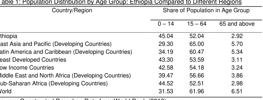
While the age distribution of the population discussed above generally characterizes developing countries with high fertility and high mortality, these figures for Ethiopia were somewhat disgusting. Table 1 compares the percentage shares of the Ethiopian population in different age groups (averaged over the years 1980 to 2009) to the corresponding average shares of the world and major developing regions of the world.
As shown in Table 1, the share of children aged 0 to 14 years in the Ethiopian
population was by far above the world average. In fact, the proportion of Ethiopia‟s
youth was above the average for any developing region in the world. In contrast, Ethiopia had the smallest share of the working age population as well as the elderly as compared to any developing region of the world and the world as a whole.
Figure 3: Population pyramid of Ethiopia by sex
14
Table 1: Population Distribution by Age Group: Ethiopia Compared to Different Regions
Country/Region Share of Population in Age Group
0 – 14 15 – 64 65 and above
Ethiopia 45.04 52.04 2.92
East Asia and Pacific (Developing Countries) 29.30 65.00 5.70
Latin America and Caribbean (Developing Countries) 34.19 60.47 5.34
Least Developed Countries 43.30 53.59 3.11
Low Income Countries 42.58 54.18 3.24
Middle East and North Africa (Developing Countries) 39.47 56.66 3.86
Sub-Saharan Africa (Developing Countries) 44.52 52.51 2.98
World 31.53 61.96 6.51
Source: Constructed Based on Data from World Bank (2010)
Inherent in such an age distribution, Ethiopia had a higher dependency ratio compared to most parts of the world. From the latest data of CSA (CSA, 2007), the age-dependency-ratio was around 93 percent. That is, under an extremely hypothetical scenario where everyone in the working age is working, a group of 100 working-age people should support extra 93 people (a total of 193 people). Under the actual situation where about 25.6 percent of the working-age population was inactive (CSA, 2007), about 20.5 percent of the labor force was unemployed (World Bank, 2010), and the
majority of those employed – around 80% – were found in low productivity subsistence
agriculture (Gete et al., 2007), the dependency ratio may have understated the burden.
Population Growth and Human Development Index
The effect of population growth on the economic performance of a country or a region is also reflected in changing HDI, which is designed to particularly reflect long-term changes in human development as opposed to short-term fluctuations. HDI comprises of measures of achievement in education, in health as well as decent standard of living.
15
Figure 4: Ethiopia compared to various groups of countries based on (A) HDI score and (B) population growth rate.
Source: Constructed Based on Data from UNDP (2011) and World Bank (2010)
In terms of growth, Ethiopia‟s HDI grew by about 27.9 percent between 2000 and 2011,
16
among the top movers in their HDI. In the report, Ethiopia was the eleventh top improver in the past forty years in terms of HDI and the eighth in terms of non-income HDI. UNDP attributed this improvement mainly to big gains made in education and public health.
As to the big gains made in education, I argue that the gain has been in numbers at the expense of quality. During our early school days, we used to consider spelling our names correctly as the first success. The recent phenomenon, however, is very horrible. The number of tertiary level students who do not spell their names correctly is not trivial. I had personally witnessed students who spell their names differently on question
papers and answer sheets. It was more awful to see master‟s students (among the
better off and chosen to be university instructors) calculating firm profit as the difference between average revenue and marginal cost, after following the course Managerial Economics for four months. Such observations had been common and too many to list.
However, the reflection these observations give to our “big educational achievements” is
very crucial. Though such facts may not be enough to deny achievements in education, they should warn us against dancing too much in celebrations.
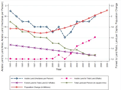
Population Growth and Pressure on Land
Another important area that reflects the effects of population growth is the pressure on natural resources like land and forests. With a rapidly increasing population, the demands for agricultural land and for energy sources would cause deforestation for expanding agricultural land and drive down the size of arable land per person and forest coverage. Besides, such a pressure induces movement to previously uncultivable land. Such population-induced movement to marginal land is unlikely to be a lasting solution since the continued population explosion will eventually inevitably lead to a situation where such a movement becomes impossible.
17
Figure 5: Population change and the pressure on land
Source: Constructed Based on Data from World Bank (2010)
Figure 5 also depicts the contrasting trends taken by population change and forest coverage of the country, especially since 1998. Again, in sharp contrast to the trend of population change, the share of forestland in total land area was declining sharply. Forest coverage fell by about 14.4 percent in fourteen years.
To sum up, the descriptive analysis showed that population growth rate is negatively associated with per capita land holding, forest coverage and HDI. However, such associations do not establish causality, the concern of the remainder of this section.
Population and Real GDP per Capita: An Econometric Analysis
This sub-section presents the econometric investigation of the relationship between population and income. While each report of UNDP has some observations of HDI, the fact that these are not comparable across reports prohibited using HDI in regression.
18
population density, employment, dependency ratio, domestic investment, human capital and openness. Table 2 summarizes the results.
Real GDP per capita, investment, human capital and openness are non-stationary in levels and log-levels, but stationary in differences and log-differences. Thus, each of these variables is I(1) while their differences and log-differences are I(0). For ease of interpretation, log-differences of these variables were preferred to differences.
19
Table 2: DFGLS and KPSS Unit Root Test Results
Variable Form
DFGLS test KPSS test
with trend without trend with trend without trend
Population Level 0.514 [5] -1.323 [2] 0.559 [2]*** 2.21 [2]***
log-level 0.203 [2] -0.062 [9] 0.573 [2]*** 2.34 [2]***
Difference -3.209 [1]** -1.562 [1] 0.244 [3]*** 1.89 [2]***
log-difference -6.855 [1]*** -0.626 [4] 0.0197 [2] 1.35 [2]***
RGDPPC Level -1.349 [2] 1.889 [1] 0.227 [2]*** 0.878 [2]***
log-level -1.029 [1] 1.410 [1] 0.262 [2]*** 0.931 [2]***
Difference -2.560 [1] -2.13 [1]** 0.249 [2]*** 0.301 [2]
log-difference -2.883 [1]* -2.040 [1]** 0.206 [3]** 0.206 [3]
INVEST Level -3.056 [1]* -1.515 [1] 0.147 [2]** 1.14 [2]***
log-level -2.057 [1] -0.498 [1] 0.261 [2]*** 1.28 [2]***
Difference -5.544 [2]*** -5.915 [2]*** 0.0361 [2] 0.0417 [2]
log-difference -4.154 [1]*** -2.990 [1]*** 0.0771[3] 0.22 [3]
Employment Level -0.787 [1] 1.354 [1] 0.513 [2]*** 2.12 [2]***
log-level -0.309 [1] 1.428 [1] 0.523 [2]*** 2.28 [2]***
Difference -2.098 [1] 0.583 [2] 0.352 [2]*** 1.76 [2]***
log-difference -4.640 [1]*** -2.539 [1]** 0.0945 [2] 1.41 [2]***
Dependency Level -2.222 [2] -1.381 [1] 0.341 [2]*** 1.18 [2]***
Ratio log-level -2.186 [2] -1.683 [2]* 0.349 [2]*** 1.18 [2]***
Difference -2.031 [1] -1.733 [1]* 0.225 [2]*** 0.837 [2]***
log-difference -1.996 [1] -1.683 [1]* 0.23 [2]*** 0.879 [2]***
HUMAN Level -1.564 [1] 0.595 [1] 0.352 [2]*** 1.85 [2]***
log-level -2.761 [1] 0.932 [1] 0.124 [2]* 2.19 [2]***
Difference -5.691 [1]*** -5.449 [1]*** 0.0399 [2] 0.2 [2]
log-difference -5.921 [1]*** -5.582 [1]*** 0.0387 [2] 0.0391 [2]
OPEN Level -1.113 [1] 1.233 [1] 0.206 [2]** 1.37 [2]**
log-level -1.114 [1] 1.137 [1] 0.287 [2]*** 1.47 [2]***
Difference -4.399 [1]*** -4.099 [1]*** 0.164 [3]** 0.176 [3]
log-difference -4.158 [1]*** -1.901 [2]* 0.153 [3]** 0.183 [3]
EMPLGR Level -4.640 [1]*** -2.539 [1]** 0.0945 [2] 1.41 [2]***
log-level -5.111 [1]*** -2.777 [1]*** 0.0737 [2] 1.45 [2]***
Difference -6.499 [1]*** -5.076 [1]*** 0.0288 [3] 0.0369 [3]
log-difference -6.035 [1]*** -3.798 [1]*** 0.0303 [3] 0.0381 [3]
POPGR Level -6.855 [1]*** -0.626 [4] 0.0197 [2] 1.35 [2]***
log-level -6.180 [3]*** -0.448 [4] 0.0228 [2] 1.37 [2]***
Difference -5.948 [7]*** -5.982 [7]*** 0.0144 [2] 0.0144 [2]
log-difference -7.639 [3]*** -7.635 [3]*** 0.0145 [2] 0.0145 [2]
20
Population density, another demographic variable, is non-stationary in all the four forms. Through subsequent tests for higher order of integration, it was found to be integrated of order two in its log, meaning that its growth rate was an I(1) variable. Stationarity for dependency ratio could not be secured up to three orders. However, this is unlikely to create any problem since total population after controlling for employment (number of workers), captures the effect of the dependent population.
In sum, the tests of stationarity indicated that the following variables were I(1), with the potential for co-integrating relationship(s): GDP per capita, domestic investment, human capital, openness, population growth rate, and growth rate of employment.
The next step was to assess the relationship among the variables in the short run and
the long run. Accordingly, Johansen‟s test of co-integration amongst the I(1) variables
was checked, first in bivariate and then in multivariate settings. In the bivariate case, the test involved the pairs RGDPPC and POPGR, and RGDPPC and EMPLGR.
With regard to the relationship between POPGR and RGDPPC, SBIC, FPE and HQIC chose lag 1 while AIC chose lag 2 as the optimal lag when tested with constant both in the differenced VAR model and in the integrating equation. With trend in the integrating equation as well as with trend in both the differenced VAR and the co-integrating equation, all the information criteria chose lag 2, with the exception of SBIC
(which chose lag 1). Consensus between Johansen‟s test and Saikkonen and Lütkepohl
21
Table 3: Estimation Results of the Bivariate VECM of ln(RGDPPC) and POPGR
Regressors ↓ Dependent Variable
∆ln(RGDPPC) ∆POPGR
ECTt-1 – 0.031 (0.011) – 0.006 (0.000)
∆ln(RGDPPC)t-1 – 0.287 (0.018) 0.017 (0.065)
∆ln(RGDPPC)t-2 0.076 (0.538) 0.016 (0.085)
∆POPGRt-1 2.069 (0.191) 0.588 (0.000)
∆POPGRt-2 5.158 (0.002) 0.187 (0.138)
DERG – 0.046 (0.014) – 0.0004 (0.797)
EPRDF – 0.007 (0.724) – 0.005 (0.001)
Constant 0.290 (0.006) 0.051 (0.000)
ECT = ln(RGDPPC) – 0.073*Trend + 181.039*POPGR
(.) (0.000) (0.000)
Note: Numbers in ( ) are p-values. This holds for Tables 4 and 5 as well.
In the co-integrating equation, the coefficient of ln(RGDPPC) was normalized to one.
The alternative of normalizing the coefficient of population growth rate yielded unreasonable estimates of adjustment parameters, and hence dropped. According to the result in Table 3, there existed a negative long run relationship between per capita
income and population growth rate. The ∆ln(RGDPPC) equation exhibits a yearly
adjustment of about 3.1% to disequilibrium in the long run relationship. The ∆POPGR
equation, on the other hand, corrects about 0.6% of disequilibrium in a year. As both equations in the VECM have statistically significant adjustment parameters (reflected in small p-values), the long run causality runs in both directions: higher rate of population growth hampers the level of per capita income, and higher level of per capita income reduces the rate of population growth. Moreover, the growth rate of GDP per capita during the Derg regime was significantly below that of the Imperial regime. Similarly EPRDF experienced by reduced changes in population growth rate than the Imperial.
There is unidirectional causality in the short run – only population growth
granger-caused real GDP per capita. As the Orthogonal Impulse Response Functions (OIRFs) suggest a stabilized causality in opposite direction materials only after a lag of 16 years.
Investigating the bivariate relationships between growth rate of employment and real GDP per capita followed, repeating steps paralleling the forerunning investigation. In this case, AIC and FPE favored lag 1 as the optimal lag while HQIC and SBIC chose lag 0. As both variables have been proved to be I(1), the former is taken. Agreement
between the two tests of co-integration favored two models – one with and the other
22
Table 4: Estimation Results of the Bivariate VECM of ln(RGDPPC) and EMPLGR
Regressors ↓ Dependent Variable
∆ln(RGDPPC) ∆EMPLGR
ECTt-1 – 0.655 (0.611) – 0.762 (0.000)
∆ln(RGDPPC)t-1 – 0.361 (0.003) 0.005 (0.691)
∆EMPLGRt-1 0.136 (0.908) 0.315 (0.011)
DERG – 0.001 (0.016) 0.0002 (0.005)
EPRDF 0.001 (0.193) 0.0002 (0.000)
Constant – 0.020 (0.830) – 0.054 (0.000)
ECT = EMPLGR – 0.015ln(RGDPPC)
(0.106)
Hence, there exists a positive long run relationship between per capita income and growth rate of employment. In this case, causality is unidirectional: from income per capita to growth of employment. Whenever the system is above or below the long run
equilibrium, the only responsive variable – ∆EMPLGR – will take the system back to
equilibrium. The speed of adjustment is about 76% per year. The regime dummies (which show trend shifts, as opposed to level shifts in Table 3) indicate that both the Derg and EPRDF regimes are better in terms of employment growth while the Derg regime is worse in terms income growth than the Imperial regime.
In the short run, neither the growth of employment granger-causes per capita income nor per capita income granger-causes the growth rate of employment. That is, short run changes in employment growth result from exogenous shocks to itself or from disequilibrium in the system and not directly from short run changes in GDP per capita. The OIRFs also suggest a weak (at 10% significance level) long-run unidirectional causality running from income to employment growth.
Next, a VECM of three variables – ln(RGDPPC), POPGR and EMPLGR – was
estimated. Pre- and post-estimation tests and the information criteria used earlier, chose the model with four lags and trend in the co-integrating equation. Despite
differences in the numerical values, two long run causalities – a negative one running
from population growth to per capita income and a positive one running from income to
employment growth – are intact (see the OIRFs). Besides, now employment growth
happens to granger-cause population growth positively (perhaps through the better prospect employment entails encouraging marriage and birth).
23
significance of the error correction term (ECTt-1) in the POPGR equation reveals that
[image:24.612.66.547.219.524.2]population growth is endogenous to the system. Thus, if income is large or employment growth is slow (or some combination of the two), the system will be above equilibrium and population growth must fall as the system gravitates back to equilibrium. However, as the speed of adjustment for this variable is very small (1% a year), its movement towards the equilibrium might be veiled (particularly by that of income).
Table 5: Estimation Results of the VECM of ln(RGDPPC), POPGR and EMPLGR
Regressors ↓ Dependent Variable
∆ln(RGDPPC) ∆POPGR ∆EMPLGR
ECTt-1 – 0.115 (0.000) – 0.010 (0.001) – 0.009 (0.014)
∆ln(RGDPPC)t-1 – 0.508 (0.000) 0.016 (0.150) 0.021 (0.141)
∆ln(RGDPPC)t-2 – 0.052 (0.648) 0.027 (0.013) 0.029 (0.041)
∆ln(RGDPPC)t-3 0.044 (0.708) 0.020 (0.069) 0.027 (0.061)
∆ln(RGDPPC)t-4 – 0.155 (0.188) 0.007 (0.536) 0.020 (0.171)
∆POPGRt-1 15.274 (0.001) 0.901 (0.032) 1.383 (0.013)
∆POPGRt-2 23.127 (0.000) 0.292 (0.451) 0.518 (0.310)
∆POPGRt-3 16.951 (0.000) 0.168 (0.639) – 0.085 (0.858)
∆POPGRt-4 10.313 (0.001) – 0.182 (0.548) – 0.319 (0.425)
∆EMPLGRt-1 – 7.896 (0.001) – 0.374 (0.108) – 0.834 (0.007)
∆EMPLGRt-2 – 13.584 (0.000) – 0.232 (0.349) – 0.479 (0.144)
∆EMPLGRt-3 – 12.724 (0.000) – 0.071 (0.784) 0.226 (0.506)
∆EMPLGRt-4 – 7.468 (0.003) – 0.012 (0.960) 0.159 (0.603)
EPRDF 0.001 (0.931) – 0.003 (0.078) – 0.001 (0.275)
DERG – 0.057 (0.016) 0.002 (0.002) 0.003 (0.002)
Constant 0.928 (0.000) – 0.075 (0.001) – 0.071 (0.016)
ECT = ln(RGDPPC) – 0.032*Trend – 58.557*EMPLGR + 166.73*POPGR
(.) (0.000) (0.000) (0.000)
With regard to short run granger-causality, GDP per capita is exogenous consistent with earlier bivariate analyses. It takes more six years before GDP per capita affects employment growth sustainably and more than five decades before it affects population growth directly and significantly.
24
two regime dummies included in addition to population growth, employment growth, and ln(RGDPPC), there existed a meaningful long run relationship among these variables.
[image:25.612.67.571.312.586.2]Like the previous VECM results, the long run relationship in this equation revealed a negative association of bidirectional causality between per capita income and population growth. This is evident from the sign of the coefficient of POPGR in the co-integrating equation and significance of the adjustment coefficients (Table 6). Thus, a slower (faster) population growth both raises (lowers) per capita income and results from a rise (fall) in per capita income. Similarly, there is a positive relationship between income per capita and growth of employment. That is, higher (lower) per capita income elevates (reduces) growth employment, which enhances the rise (fall) in per capita income. Furthermore, increase in domestic investment raises real GDP per capita and this in turn brings about a rise in domestic investment in the long run.
Table 6: Estimation Results of the Full Multivariate VECM
Regressors ↓ Dependent Variable
∆ln(RGDPPC) ∆ln(INVEST) ∆EMPLGR ∆POPGR ∆ln(OPEN)
ECTt-1 -0.105*** -0.333** -0.016*** -0.020*** -0.089
∆ln(RGDPPC)t-1 -0.334** 0.628 0.036** 0.034*** 1.008***
∆ln(RGDPPC)t-2 0.087 -0.937* 0.002 0.017 0.001
∆ln(INVEST)t-1 0.012 -0.368** -0.008* -0.005 -0.265***
∆ln(INVEST)t-2 0.034 0.153 0.008* 0.002 -0.114***
∆EMPLGRt-1 -2.813 4.774 -0.586** -0.293 -0.959
∆EMPLGRt-2 -5.728*** -8.590 -0.551** -0.143 6.358*
∆POPGRt-1 4.393 8.048 1.150*** 0.942*** 6.717
∆POPGRt-2 11.122*** 17.385 0.611* 0.351 -1.825
∆ln(OPEN)t-1 -0.006 0.0931*** 0.010 0.006 0.037
∆ln(OPEN)t-2 0.185*** 0.351 -0.002 0.002 0.197*
DERG -0.023 -0.046 0.003 0.003** -0.011
EPRDF 0.054*** 0.005 0.005** 0.005*** -0.006
Constant 0.059*** 0.228*** 0.007*** 0.008*** 0.076**
ECT = ln(RGDPPC) – 0.181OPEN – 0.283ln(INVEST)*** – 28.048(EMPLGR) *** + 88.557(POPGR) ***.
Note: *, ** and *** depict significance at 10%, 5% and 1% significance level, respectively.
25
Granger-causality tests support lack of instantaneous causality running from openness and employment growth to the other variables. OIRFs were used to assess the dynamics of how shocks to each of the variables affect all the variables. The OIRFs for this full model show that an orthogonal shock to population growth will induce a significant reduction in per capita income (at 5% level) and openness (at 10% level) and a significant rise in employment growth with a lag of close to two decades (at 5% level). A shock to GDP per capita induces a slowdown in population growth rate with a lag of more than a decade and a half, and a permanent boost to itself. Though OIRFs support bidirectional causality between GDP per capita and population growth, causality from the latter to the former is stronger and robust to a number of alternative specifications.
Shocks to employment growth enhance investment and population growth. Shocks to openness appear to have significant positive effects on GDP per capita and investment, and less significant positive effect on population and employment growth rates. Finally, shocks to investment appear not to have a significant effect on any other variable (except itself), though this is in contrast to the significant positive effect it had on income per capita suggested by the co-integrating equation.
To sum up, there is a significant negative relationship between population growth and the economic performance of Ethiopia in the long run, but not in the short run. Significant and robust bidirectional causality characterizes the long run relationship between population growth and GDP per capita. The short run relationship between growth rate of GDP per capita and change of population growth, however, looks unidirectional (from population to income) but not robust to alternative specifications. Changes in sign and/or significance occur from one model to another. As the models have controlled for the growth of employment, this relationship between population growth and per capita income reflects the impacts of (and the effects on) the growth of the dependent population. The growth of employment has a positive and significant long run relationship with per capita income, with bidirectional causality. Again, the short run relationship is not robust to alternative model specifications.
26
SUMMARY AND CONCLUSION
This paper examined the interrelationship between demographic variables and economic performance of Ethiopia. Using the VECM approach and controlling for openness, domestic investment and regime changes, it assessed the direction and strength of causality between the growth rates of population and workers on the one hand and the level of real GDP per capita on the other. Besides, it supplemented the econometric investigation with descriptive analysis highlighting the pressure of population change on the HDI, agricultural land and forest coverage of the country.
The population of Ethiopia more than quadrupled in about six decades. Though there was some tendency of stabilizing/declining rate of population growth, this is far from an accomplishment as the absolute change in population continued to rise. With most of its population at the bottom of population pyramid, the working-age population accounted for slightly above half of the total. The share of children below the working-age in the Ethiopian population was by far above the world average and the average for any developing region. While the very high average rate of natural increase played the dominant role in shaping the demographic dynamics of Ethiopia, international migration also played significant roles particularly during periods of political instability.
In contrast with the position of the country in terms of population growth, Ethiopia registered HDI scores that are by far less than even the average for low-human-development countries. Despite some improvement in HDI, the rising numbers might have come at the expense of quality (especially in education). However, denying claims of improvements wholly might carry danger of political prejudice. Also evident from the descriptive analysis, population growth had inverse relationship with per capita land holding, total forest coverage, and HDI score of the country.
The econometric analysis of the VECM relating population and real GDP per capita, suggested existence of bidirectional causality between demographic and economic variables. Rises in per capita income reduced the growth rate of population and enhanced the growth rate of employment, and vice versa. Similarly, slowed growth rate of the population and/or faster growth rate of employment enhanced the betterment of real income per person. Short run relationships were, however, not robust to alternative model specifications.
All the findings point to a better attention – on the side of the government – to issues of
27
population that accounted for about 84% of the country‟s population. Secondly, efforts in
areas such as microfinance should be encouraged and extended so that women would be economically empowered, and would subsequently have more saying in family decisions like fixing the desired family size. Finally, teaching the benefits of small family size particularly to the majority in the rural should be given due attention.
REFERENCES
Baum C (2000). KPSS: Stata Module to Compute Kwiatkowski-Phillips-Schmidt-Shin Test for Stationarity. Statistical Software Components with number S410401. Boston College Department of Economics, Revised 26 June 2006. Retrieved
on March 26, 2012 from http://fmwww.bc.edu/repec/bocode/k/kpss.ado and
http://fmwww.bc.edu/repec/bocode/k/kpss.hlp
Birdsall N (1988). Economic Approaches to Population Growth. In: Chenery H,
Srinivasan T (1988). (eds). Handbook of Development Economics, Volume I.
Elsevier Science Publishers B.V.
Bloom D, Canning D, Sevilla J (2001, December). Economic Growth and the Demographic Transition. NBER Working Paper No. 8685. MA, Cambridge Bloom D, Canning D, Fink G, Finlay J (2007, May). Realizing the Demographic
Dividend: Is Africa any different? Program on the Global Demography of Aging, Harvard University
CSA (2007). The 2007 Population and Housing Census of Ethiopia: Statistical Report at Country Level. The Office of Population Census Commission: Addis Ababa. Darrat A, Yousif Y (1999). On the Long-Run Relationship between Population and
Economic Growth: Some Time Series Evidence for Developing Countries. Eastern Economic Journal, Vol. 25, No. 3, pp. 301-313.
Ehrlich I, Lui F (1997). The problem of population and growth: A review of the literature from Malthus to contemporary models of endogenous population and endogenous growth. Journal of Economic Dynamics and Control, 21, pp 205-242. Elsevier Science B. V.
Fisher S, Newman K (2011, September). Population and the MDGs: The Missing Link. Freedom from Want, Vol. 1, Issue 3. Asian Institute of Technology. Available
at: www.arcmdg.ait.asia/FFW3.pdf
Gete Z, Trutmann P, Aster D (2007). (eds.). Fostering New Development Pathways: Harnessing Rural-urban Linkages (RUL) to Reduce Poverty and Improve Environment in the Highlands of Ethiopia. Proceedings of a Planning Workshop on Thematic Research Area of the Global Mountain Program
(GMP) held in Addis Ababa, Ethiopia, August 29-30, 2006. Global Mountain
28
Heston A, Summers R, Aten B (2011, May). Penn World Table Version 7.0, Center for International Comparisons of Production, Income and Prices at the
University of Pennsylvania. Available Online at:
http://pwt.econ.upenn.edu/php_site/pwt62/pwt62_form.php.
Keller E (2009). "Ethiopia." Microsoft®Student 2009 [DVD]. Redmond, WA: Microsoft Corporation, 2008.
Kelley A (2001). The Population Debate in Historical Perspective: Revisionism Revised. In: Birdsall N, Kelley A, Sinding S (eds.) Population Matters: Demographic Change, Economic Growth, and Poverty in the Developing World. Oxford
University Press, pp. 24–54.
Kelley A, Schmidt R (1995). Aggregate Population and Economic Growth Correlations: The Role of the Components of Demographic Change. Demography, 32:543-55.
Keskinen M (2008). Population, Natural Resources and Development in the Mekong: Does High Population Density Hinder Development? In: Kummu M, Keskinen M, Varis O (eds.). Modern Myths of the Mekong, pp. 107-121. Water and Development Publications, Helsinki University of Technology Latimer A, Kulkarni K (2008, July-December). Population Explosion and Economic
Development: Comparative Analysis of Brazil and Mexico. Knowledge Hub, the Journal of Rajiv Academy for Technology and Management (RATM), Vol. 4, No. 2, pp. 57-70. U. P.: India
Macro International Inc. (2007, January). Trends in Demographic and Reproductive Health Indicators in Ethiopia: Further Analysis of the 2000 and 2005 Demographic and Health Surveys Data. Calverton, Maryland USA.
Mankiw N, Romer D, Weil D (1992). A Contribution to the Empirics of Economic Growth.
QJE, 107(2): 407–437.
Merrick T W (2002, March). Population and Poverty: New Views on an Old Controversy.
Vol 28, No 1, pp 41 – 46, International Family Planning Perspectives.
MoFED (2006, September). Ethiopia: Building on Progress. A Plan for Accelerated and Sustained Development to End Poverty (PASDEP) (2005/06-2009/10). Volume I: Main Text. Addis Ababa.
Moneta A, Chlass N, Entner D, Hoyer P (2011). Causal Search in Structural Vector Autoregressive Models. JMLR: Workshop and Conference Proceedings 12,
pp. 95–118
Nafziger E (2006). Economic Development, Fourth Edition. Cambridge University Press,
New York.
Panayotou T (2000, July). Population and Environment. CID Working Paper No. 54 Environment and Development Paper No.2
29
Ringheim K, Teller C, Sines E (2009, December). Ethiopia at a Crossroads: Demography, Gender, and Development. PRB Policy Brief.
StataCorp (2009). Stata: Release 11. Statistical Software. College Station, TX: StataCorp LP.
Singh D, Singh S (1997). Population Growth and Development Relationship: A Critique. In: Singh A, Rai V, Mishra A (eds.) Strategies in Development Planning. Deep and Deep. pp. 368-388.
Todaro M, Smith S (2006). Economic Development, 9th ed. Boston: Addison Wesley
Publishers.
UN (2011a). World Population Prospects: The 2010 Revision, CD-ROM Edition, New York: Population Division of the Department of Economic and Social Affairs. UN (2011b). World Fertility Policies 2011. New York: Population Division of the
Department of Economic and Social Affairs.
UNDP (2010). Human Development Report 2010 – The Real Wealth of Nations:
Pathways to Human Development. 20th Anniversary Edition. New York:
Human Development Report Office.
UNDP (2011). Human Development Report 2011 – Sustainability and Equity: A Better
Future for All. New York: Human Development Report Office.
UNFPA (2011). The State of World Population 2011. People and Possibilities in a World of 7 Billion. New York: Information and External Relations Division.
World Bank (2010). World Development Indicators and Global Development Finance,
February 17, 2011 Revision. Washington D. C. The World Bank.
Yousif H (2009). How Demography Matters for Measuring Development Progress in