Stochastic Volatility in the U S Labor Market

Munich Personal RePEc Archive

Stochastic Volatility in the U.S. Labor

Market

Dennis, Wesselbaum

University of Hamburg, German Physical Society, EABCN

29 November 2012

Online at

https://mpra.ub.uni-muenchen.de/43054/

Stochastic Volatility in the U.S. Labor Market

Dennis Wesselbaumy

University of Hamburg, German Physical Society, and EABCN

November 29, 2012.

Abstract

In state-of-the-art macroeconomic and labor market models shocks are assumed to be ho-moscedastic. However, we show that this assumption is much too restrictive. We …nd signi…cant evidence for strong time-varying volatility in all considered labor market time series.

First, we estimate theunconditionalvariance-covariance matrix and …nd signi…cant evidence for time variability. Second, we estimate theconditional variance-covariance matrix and discuss the time-varying risk contained in labor market variables.

The implications are relevant for modelling purposes, welfare analysis, and the understanding of sources of ‡uctuations.

Keywords: Dynamic Correlation, Multivariate GARCH, Stochastic Volatility. JEL codes: C30, E30, J60.

I would like to thank Ester Faia and Uwe Hassler for highly useful comments and discussions. All remaining errors are my own.

y_{University of Hamburg, Chair of Computational Economics, Von-Melle-Park 5, 20146 Hamburg, Germany. Email:}

1

Introduction

In macroeconomic models dynamic e¤ects of shocks are simulated by imposing the ad hoc assump-tion of homoscedasticity of the underlying stochastic processes. However, recent research has shown that various macroceconomic time series exhibit a strong time-varying variance with clustering of periods with high and low volatility. Sims and Zha (2006) use a structural vector autoregression model allowing for Markov regime switching and show that the best …t is obtained with a model that features time-varying variances of structural disturbances. More recently, Fernandez-Villaverde and Rubio-Ramirez (2010) estimate the stochastic volatility present in aggregate time series and the estimation by Justiniano and Primiceri (2008) show a strong stochastic volatility of shocks in the United States that vary considerably across types of shocks.

A di¤erent, though related issue is the role played by uncertainty. Higher volatility of variables that in‡uence the optimization problem of economic agents can have substantial e¤ects on the optimal path of actions. This is especially important in the presence of non-convex adjustment costs, irreversibilities, or non-linearities in the production set. Bloom (2009) and Bloom et al. (2012) show that higher risk may lead a household to defer investments because of the fear to hit a liquidity or credit constraint that may impact the optimal consumption allocation in the future. Along this line, an increase in the volatility, for example, of the job separation rate may lead the household to increase savings out of precautionary motives or a¤ect its e¤ort and hence her productivity. Therefore, (increased) volatility in labor market variables can have substantial real e¤ects.

While there is extensive evidence for macroeconomic time series, there is only very sparse evi-dence concerning labor market variables. Stock and Watson (2002) use time series for employment, unemployment, wages, and the help-wanted index and estimate an AR(4) process to address the change in the (time-varying) standard deviation. They …nd a signi…cant time-varying component but they neither report the behavior of the unconditional mean of variance and covariance nor do they estimate the dynamic interdependencies between those variables.

In order to fully understand the source of ‡uctuations in the labor market, for welfare analysis, and for policy advice it is, however, important to consider all time series that are present in the workhorse labor market model, the Mortensen-Pissarides (1994) search and matching model. This paper aims at providing this missing empirical evidence.

The purpose of this paper is to discuss the stochastic volatility of labor market variables in the United States and hence is purely descriptive. We will leave a (micro)foundation of the observed stochastic volatility to future research. The contribution of this paper is twofold. First, we estimate the unconditional mean of the variance and covariance for the U.S. labor market to address the assumption of homoscedasticity in macroeconomic and, in particular, in labor market models. Here, we estimate a time-varying parameter VAR model as in Primiceri (2005). We …nd signi…cant evidence for time variability in the unconditional mean and in the unconditional correlation.

Second, we estimate the conditional variance and covariance and therefore are able to analyze the behavior of uncertainty in the labor market. We do so by estimating a multivariate generalized ARCH model, namely the dynamic conditional correlation model proposed by Engle (1999). This model allows for stochastic variance and stochastic correlations and is therefore able to shed light on the behavior of the conditional second moments over time. We …nd that labor market variables contain large amount of time-varying risk.

macro-and labore economists should be interested in second moments as well. As discussed in detail in Hamilton (2008), misspeci…cation of the variance-covariance matrix will make a hypothesis test on the mean invalid. Further, e¢ciency in estimating the …rst moments can be increased by including the observed heteroscedasticity. Moreover, time-varying …rst and second moments can be seen as evidence for non-linearities in the economy.

The paper is structured as follows. The next section discusses our data set. Section 3 will discuss the estimation of the unconditional variance-covariance, while section 4 will deal with the estimation of the conditional variance-covariance matrix. Section 5 concludes.

2

Data

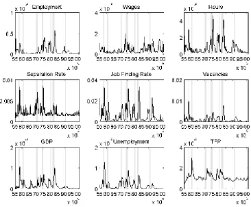
In the subsequent chapters we will use di¤erent labor market time series, namely employment, vacancies, unemployment, wages, total factor productivity (TFP, for short), (job) separation rate, job …nding rate, hours, and the gross domestic product (GDP, for short). All time series are seasonally adjusted and are on a quarterly basis and cover the period from 1955:Q1 to 2000:Q4, which gives us 184 data points.

For section 3 of this analysis, we use the un…ltered time series, while for section 4 we pass the time series through a Hodrick-Prescott …lter with smoothing parameter 1600 in order to obtain the necessary zero-mean input series (see section 4 for more details).

Employment is measured by the number of nonsupervisory workers as constructed by the Bureau of Labor Statistics (BLS, for short). The series for vacancies is constructed from the help-wanted advertising index by the Conference Board. Unemployment is measured by the unemployment rate as published by the BLS in its Current Population Survey (CPS, for short). For wages we use the real hourly compensation series from the BLS.

The time series for TFP is taken from Basu et al. (2006) and is utilization-adjusted TFP for the U.S. Business Sector. For the separation rate and the job …nding rate, we use the time series constructed by Shimer (2012) from employment, unemployment, and mean unemployment duration. The quarterly time series are averages of monthly rates.

Hours are constructed as the average weekly hours worked by all persons in nonfarm business multiplied by civilian employment and normalized by the labor force. All time series obtained by the BLS with the exception being average weekly hours being taken from the U.S. Department of Labor. Finally, the time series for GDP is taken from the NIPA tables.

3

Estimating the

Unconditional

_{Variance-Covariance Matrix}

This section is concerned with the estimation of the unconditional mean of the variances and covariances of our time series. In order to do so, we will review the time-varying parameter VAR model developed in Primiceri (2005).

3.1 Model

Let _fytg denote a N 1 dimensional vector of random variables and assume that the N

1 dimensional vector ct contains time-varying coe¢cients. Further, denote N N dimensional

matrices of time-varying coe¢cients byBi;t; i= 1; : : : ; k, wherek determines the lag length. Then, the model can be written as

yt=ct+B1;tyt 1+: : :+Bk;tyt k+ut; t= 1; : : : T; (1)

whereT is the sample size. Here, we assume that the exogenous disturbances, ut, have a

variance-covariance matrix t.

Using this variance-covariance matrix and applying a triangular factorization, we …nd

At tA0_t= t 0t; (2)

where we denote the diagonal matrix with t

t= 2 6 6 6 6 4

1;t 0 : : : 0

0 2;t . .. ...

..

. . .. ... 0 0 : : : 0 N;t

3 7 7 7 7 5 ; (3)

with i;t >0; 8 i= 1; : : : ; N.

Further, At is a lower triangular matrix with ones a long the main diagonal and zeros above the main diagonal elements

At= 2 6 6 6 6 4

1 0 : : : 0

2;1;t 1 . .. ...

..

. . .. . .. 0

N;1;t : : : N;N 1;t 1

3 7 7 7 7 5 : (4)

Then, we can write the model in eq. (1) as

yt = ct+B1;tyt 1+: : :+Bk;tyt k+A

1

t t"t; t= 1; : : : T; (5)

V("t) = IN; (6)

where V("t) is the variance-covariance matrix of the disturbances and IN is a N dimensional

identity matrix. Finally, we can write the model as

yt = X0tGt+At1 t"t; (7) X0_t = IN 1; y0t 1; : : : ; y0t k ; (8)

whereGtis a vector that stacks the entire right-hand-side coe¢cients of (5) and is the Kronecker

product operator.

In the following, we need to impose some structure on the dynamic evolution of the time-varying parameters. We do so by assuming a random walk behavior, i.e.

Gt = Gt 1+ t; (9)

at = at 1+ _t; (10)

where vectoratstacks the non-zero, non-one elements of matrixAtand vector tstacks the diagonal

elements of t. All disturbances are assumed to be Gaussian with the following variance-covariance

matrix

V=V ar

2 6 6 4 "t t t t 3 7 7 5= 2 6 6 4

IN 0 0 0

0 Q 0 0 0 0 S 0 0 0 0 W

3

7 7

5; (12)

whereQ;S;W are all positive de…nite matrices.

Finally, it is worth noticing that the ordering of variables does, to some extend, a¤ect the results. This caveat follows from the factorization in eq. (2) and the resulting lower triangular structure of At. From the literature on search and matching models, we assume the following ordering of variables in our VAR

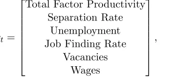
yt=

2 6 6 6 6 6 6 4

Total Factor Productivity Separation Rate

Unemployment Job Finding Rate

Vacancies Wages 3 7 7 7 7 7 7 5 ; (13)

hence - by lower triangularity - we assume that total factor productivity drives all other variables and can be considered to be the most exogenous variable. On the contrary, we assume that wages is the most endogenous variable, as all variables ordered before will have an e¤ect on it. In addition, this is not just an ordering issue but also an identi…cation issue. With this structure, we are able to isolate the productivity shocks, as they are considered to be the main driving force in the canonical search and matching model.

3.2 Estimation Results

As in Primiceri (2005), we use Bayesian methods to estimate the parameters of interest. To be precise, those are the unobservable statesBT;AT; T and the variance-covariance matrixV. The MCMC algorithm uses Gibbs sampling drawing a sample from BT;AT; T;V conditional on the data and the remaining parameters. Given this sample, a reduced form VAR of the type

yt=X0tBt+ t"t; (14)

can be estimated, that results in posteriors for B and at any given point in time.1 _{Then, the}

posterior values for t are obtained by solving the system of equations for every draw of t

t 0t= t;8t: (15)

The solution is given by

t=At1 t; (16)

because of the triangular identi…cation approach.

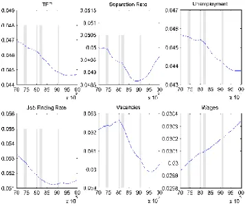
We estimate the TVP-VAR with 70.000 draws of which 20.000 are used as burn-in-draws. Further, we use the …rst 60 observations to calibrate the prior distributions. Our results are presented in Figure 1 to 3.

Figure 1 presents the unconditional variance point estimates for the six shocks considered. We observe a signi…cant and considerable amount of time variation in the time series at hand. The

1_{Identi…cation is ensured by letting}

Figure 1: Estimated unconditional standard deviations. Shaded areas indicate NBER recession dates.

volatility in TFP declines nearly linearly from 0.047 at the beginning of our sample to a value close to 0.045. We observe a similar pattern for unemployment decreasing from a value close to 0.046 to a value between 0.0435 and 0.044. Further, a similar pattern is visible for the job …nding rate. We observe a drop from 0.0535 to 0.0515 and a rough stabilization for the last 50 quarters on this level. On the contrary, we …nd that the volatility of wages has increased over the sample. Starting on a value of 0.0299 our estimation shows a …nal value of roughly 0.0304. Most interesting though is the evolution of the variances of the separation rate and vacancies. For the separation rate, we observe a sharp decline within the …rst half of the sample period from a value of roughly 0.05 to a value of 0.0486. Afterwards, in the second half of the sample, we …nd a sharp pick up of the variance reaching a value of 0.0496 at the end of the sample. Similarly, we …nd this pattern for vacancies, although less pronounced. The volatility of vacancies increases for almost 50 periods and then sharply declines for the next 50 quarters. At the end of the sample we again observe a pick up of the volatility.

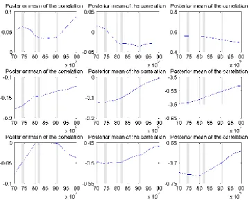
Figure 2: Estimated unconditional correlations. Shaded areas indicate NBER recession dates.

of the correlation structure between TFP and unemployment. While this correlation was positive (0.02) at the beginning of the sample, we observe that the cyclicality is reversed and after roughly 25 periods, the correlation is signi…cantly negative, e.g. we …nd a …nal value of roughly -0.03.

Moreover, we observe a stable, positive relationship between the separation rate and unemploy-ment. Moreover, we …nd a relatively stable relationship between the separation rate and the job …nding rate, vacancies, and wages. Although the correlation tends to become smaller.

The correlation between the job …nding rate and vacancies stays roughly constant over the sample period, though we observe a slight decline. The correlation between the job …nding rate and wages varies considerably over the sample. Initially, it increases for the …rst 50 periods, then declines for the next 50 quarters, increases again, but starts to decline at the end of the sample.

Finally, we …nd that the correlation of unemployment with the job …nding rate, vacancies, and wages all start to become less negative after some time. For vacancies and wages it takes roughly 50 quarters after which the correlation starts to become smaller, while it almost immediately starts to increase for the job …nding rate.

4

Estimating the

Conditional

_{Variance-Covariance Matrix}

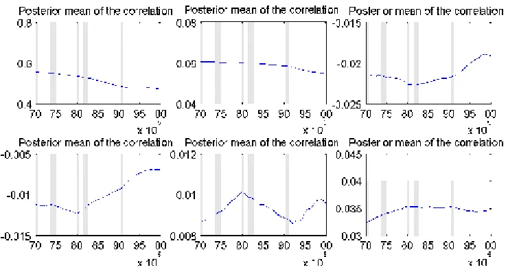
Figure 3: Estimated unconditional correlations. Shaded areas indicate NBER recession dates.

4.1 Model

Generally, let_fytgdenote aN 1dimensional vector of random variables withE[yt] = 0. Further,

let It be the smallest -…eld generated by the history of values of yt, i.e. It = (yr; r t 1).

Moreover, assume that the time series in our vector _fytg are conditionally multivariate Gaussian

with zero mean and covariance matrix Ht. By imposing measurability ofHt with respect to_Itwe

can write the multivariate GARCH as

ytjItsN (0;Ht); (17)

and, formally, yt =pHt t, where t is aN 1 dimensional vector of i.i.d. errors. The next step

is to put some structure on the N N dimensional, positive semi-de…nite, symmetric conditional covariance matrixHtand this is done by modelling the conditional variances and correlations, i.e.

Ht=DtRtDt: (18)

Here,Dt is aN N diagonal matrix of time-varying conditional standard deviations and Rt is a

N N dimensional time-varying conditional correlation matrix. The former matrix is given by

Dt=

2

6 6 6 6 4

p

h1;t 0 0

0 ph2;t . .. ...

..

. . .. . .. 0 0 0 phN;t

3

7 7 7 7 5

; (19)

wherephi;t 8 i2 f1; :::; Ng is estimated from a univariate GARCH(q; p)model.

This GARCH(q; p) model can be written the usual way as

hi;t = i;0+

q

X

j=1

i;jyi;t j2 + p

X

j=1

with i;0 > 0; i;j 0; and i;j 0 8 i; j. Further, we denote the standardized residuals as

"t=Dt1ytsN (0;Rt), where we standardize by the conditional standard deviation.

It can be shown that a necessary and su¢cient condition for stationarity of those univariate GARCH processes isPq_j=1 i;j+

Pp

j=1 i;j <1 8 i.

The symmetric correlation matrix Rt is given by

Rt=

2 6 6 6 6 4

1 1;2;t 1;N;t

1;2;t 1 . .. ...

..

. . .. . .. _N 1;N;t

1;N;t N 1;N;t 1

3 7 7 7 7 5 ; (21)

where i;j;t is the correlation estimator. We would like to ensure that Htis positive de…nite, since

it is a covariance matrix, and all elements of the correlation matrix,Rt, are less or equal to one in absolute terms.

For this purpose, it is assumed that the conditional correlation matrix follows

Rt = Q_t 1QtQ_t 1; (22)

Qt = 1 M X m=1 m K X k=1 k ! Q+ M X m=1

m"t m"0t m+ K

X

k=1

kQt k; (23)

where Q = E["t"0t] is estimated by the sample mean. Then, Qt = diag pq11;t; ;pqN N;t

re-scales the elements ofQt to ensure that the elements of the correlation matrix are less or equal to one in absolute terms, i.e. _i;j;t = qi;j;t

p_q

i;i;tqj;j;t 1. Positive de…niteness of Ht with probability

one is ensured by i;j 0; i;j 0 8 i; j, positive de…nite Q0, and the stationarity condition

Pq

j=1 i;j+

Pp

j=1 i;j <1 8 ias in Engle and Sheppard (2001).

After discussing the primitives of the model, we want to brie‡y describe the estimation strategy of the DCC model. Because we assumed our errors, _t, to be multivariate Gaussian, we can derive the joint distribution ofzt as

f( _t) =

T

Y

t=1

(2 ) N2 _e 12

0

t t_; (24)

where we used the properties of the i.i.d. shock E[ t] = 0 and E[ t 0t] =IN. Then, by using our

original de…nition,yt=pHt t, we can write the likelihood function as

L( ) =

T

Y

t=1

(2 ) N2 ₍j_Htj₎ 12_e 12yt0H

1

t yt_{; (25)}

wherejHtjis the determinant ofHt. Further, contains the parameters of the univariate GARCH

model for theith_{time series, i.e. ( ; ) = (}

1; : : : ; N; )and i = i;0; i;1; : : : ; i;p; i;1; : : : ; i;q 8 i

and = ( 1; : : : ; M; 1; : : : ; K) contains the parameters of the correlation structure.

After some algebra, the log-likelihood estimator is given by

ln (L( )) = 1 2

T

X

t=1

Nln (2 ) + 2 ln (_jDtj) + ln (jRtj) + 0tR

1

t t :

Then, the quasi maximum log-likelihood estimator is

ln (QL1( jyt)) =

1 2 N X n=1 "

Tln (2 ) +

T

X

t=1

"

log (hi;t) +

y2

i;t

hi;t

##

: (26)

The …rst stage estimator intuitively is the summation of individual log-likelihood values of univariate GARCH models for each time series in yt. The only remaining parameters to be estimated after

the …rst step are the ones contained in .

Consecutively, step two uses the correctly speci…ed likelihood

ln QL2 j^; yt =

1 2

T

X

t=1

Nln (2 ) + 2 ln (jDtj) + ln (jRtj) + 0tR

1

t t ; (27)

here, we condition on the parameters estimated in the …rst step. Due to conditioning on the estimated parameters, we could exclude the constant parameters from the maximization and only consider the latter two terms in eq. (27).

Consistency and asymptotic normality of the two step QMLE estimator has been shown by White (1996) and Engle and Sheppard (2001).

4.2 Test on Constant Correlation

Engle and Sheppard (2001) suggest a test on constant correlation that standardizes the residuals of the estimate of univariate GARCH processes. Consecutively, the correlation of the standardized residuals is estimated, jointly standardized by the symmetric square root decomposition of the correlation matrix (R 12D_t1y_t). If correlation would truly be constant, then the residuals would

be i.i.d. with an identity matrix as variance-covariance matrix. Therefore, the hypothesis is

H0 : Rt=R; (28)

vs:

Ha : vechu(Rt) =vechu R + 1vechu(Rt 1) +: : :+ _pvechu(Rt p); (29)

where vechu _{is a vech-operator that only uses elements above the diagonal. Then, the vector}

autoregression is

Yt= + 1Yt 1+: : : _sYt s+ t; (30)

whereYt=vechu R

1

2D_t1y_t R 12D_t1y_t

0

IN . Again, if the null would be true, all

regres-sion coe¢cients would be zero. Finally, the test statistic is ^X0_X^

2 , whereX contains the regressors

and^ contains the estimated regression coe¢cients. Then, the test statistic will be asymptotically

2

(s+ 1).

If we apply this test to our data, we …nd that the value of the test statistic is99:02with a p-value of0, using …ve lags. Put di¤erently, the probability that the correlation is constant is e¤ectively 0. Therefore, we reject the null hypothesis that the correlation in our data set is constant.

4.3 Model Selection

Silvennoinen and Teräsvirta (2007)). In order to judge the goodness of …t of our model, we employ the Akaike Information Criterion (AIC, for short) and search for the minimum value across models. The basic idea of the AIC is to estimate the Kullback-Leibler divergence that describes how close two probability distributions are to each other. Further, in large samples the Kullback-Leibler divergence can be estimated by the likelihood score, as the likelihood score is as an asymptotically unbiased estimator of the cross-entropy risk.

The AIC is de…ned as

AIC = 2 ln (L( ; )) + 2p; (31) wherep denotes the number of free parameters.

The …ve models considered are the Bollerslev (1990) constant conditional correlation model (CCC, for short), the dynamic conditional correlation model described in section 2, the integrated dynamic conditional correlation model (IDCC, for short)2_{, the full BEKK model by Engle and}

Kroner (1995), and the full BEKK model with t-distributed error terms (TBEKK, for short). As

Table 1: Akaike Information Criterion for the …ve di¤erent models. CCC DCC IDCC BEKK TBEKK AIC -853.82 -863.77 -853.34 -854.67 -856.33

we can infer from Table 1, the DCC model gives the lowest AIC score and hence, the next chapter discusses the results from estimating the DCC model on our data set.

4.4 Estimation Results

We begin by discussing the results of the conditional standard deviation estimation following from the DCC model. The behavior of the standard deviations is shown in Figure 4. From this …gure, we can draw several interesting conclusions.

We …nd evidence for a signi…cant decline of volatility in almost all time series which has been named the "Great moderation" and started around the mid 1980’s. However, there are two counterexamples, namely wages and the job …nding rate. For those two variables there is almost no di¤erence in their behavior before or after the starting point of the Great moderation (1984 is accepted by most researchers). In fact, it appears that wages are more volatile after 1984 than before, as we observe four large peaks and see only very small peaks from 1955 to the early 70’s. The job …nding rate is quite volatile in the …rst half of the 1990’s but seems to become much less volatile after this period of high volatility. Further, we …nd that the during the Great moderation the recession at the early 90’s had only very limited impact on the volatility of almost all variables, which is signi…cantly di¤erent to earlier recessions. Here, we observe a decoupling of recessions and peaks of volatility. Finally, the we …nd evidence that the length of the recession is uncorrelated with the size of the peak in volatility.

We can cluster variables into four groups according to the size of their ‡uctuations, i.e. their riskiness. Employment, wages, and hours show the smallest values of conditional volatility. On the ‡ipside, vacancies, the separation rate, and the job …nding rate have the largest values.

2_{Integratedness here refers to the fact that the stationarity condition now holds with equality, i.e.} Pq

j=1 i;j+ Pp

Figure 4: Estimated conditional standard deviations. Shaded areas indicate NBER recession dates.

Unemployment and TFP are more volatile as GDP but lie somewhere in between the two extremes. Further, while the volatility of all variables varies around zero, we …nd that the volatility of TFP varies around 0.001, while the separation rate varies around a level of 0.0015. In all …gures NBER recession dates are shaded in grey in order to stress the synchronicity of recessions and peaks of volatility. We observe that recessions tend to lead peaks of volatility for most variables. However, this does not hold for the separation rate, wages, and TFP. For TFP we …nd that peaks of volatility occur during recessions. Similarly, we …nd this type of behavior for the separation rate. However, there seems to be no systematic pattern between recession dates and peaks of volatility.

In general, there is an isomorphic mapping between recession dates and peaks, put di¤erently every large peak is associated with a recession and every recession is associated with a peak of volatility. However, we should be careful in mistaking correlation with causation. Along this line, it would be interesting to think about the transmission of risk of an isolated type of shock (or policy reform) onto other variables. For example, consider the peak of the volatility from the job …nding rate in the …rst half of the 90’s. A fairly large peak is visible which is also visible in other time series but not in the separation rate. This leads to the conclusion that the underlying event occurred on the entry site of the labor market, or had larger e¤ects on the (volatility of the) entry side.

Figure 5: Estimated conditional covariances. Shaded areas indicate NBER recession dates.

estimation.

As we have seen for the standard deviations, we observe the dampening e¤ects of the Great moderation and a decoupling of recessions and covariance peaks. Further, we again observe that recessions lead peaks of correlations.

However, we …nd that employment and wages are positively correlated which changes af-ter 1980, where we observe small but negative peaks. This observation also holds for the covariance of wages with vacancies and hours.

The covariance of TFP with all variables are highly volatile and switches from procyclical to countercyclical.

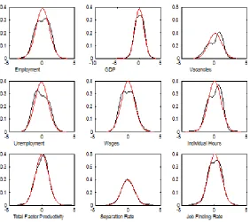
At the end of our discussion, we want to brie‡y discuss the resulting residuals from our DCC estimation. Table 2 present kurtosis and skewness values. We …nd that employment, vacancies, unemployment, and wages are platykurtotic, i.e. their distribution shows thinner tails. The re-maining variables are all leptokurtotic. Further, we …nd that employment, GDP, vacancies, hours, and the job …nding rate show left-skewed errors, while the remaining variables are right-skewed.

Figure 9: Kernel density estimation (black line) vs. normal estimation (red line) of residuals -DCC.

In order to assess whether the errors are in fact normally distributed, we use the Jarque-Bera test (JB, for short) on whether skewness and kurtosis of the distribution …ts a normal distribution with unknown moments and the Lilliefors test (LF, for short) on whether the data is from a normal distribution with unknown moments. We …nd that the JB test rejects the null of normally distributed errors for GDP, vacancies, and unemployment, while the LF test rejects the null for employment, vacancies, unemployment, wages, hours, and the job …nding rate. Both tests are performed on a 5 percent signi…cance level.

We can conclude that the errors from unemployment and vacancies are in fact non-normally distributed, while for employment, wages, hours, and the job …nding rate there is no clear evidence.

5

Conclusion

In state-of-the-art macroeconomic and labor market models the dynamic e¤ects of shocks are simu-lated by imposing the ad hoc assumption of homoscedasticity of the underlying stochastic processes. However, this assumptions seems to be arbitrary given the recent research agenda on time-varying variance in aggregate time series. Along this line, changes in volatility, or in the riskiness, in labor market variables can have substantial real e¤ects. This paper provides missing evidence on sto-chastic volatility in the U.S. labor market. Using a number of labor market time series, covering the period from 1955 to 2000, we present evidence of strong time variability. First, we estimate the

unconditional mean of the variance and covariance to address the assumption of homoscedasticity in macroeconomic and, in particular, in labor market models. Here, we estimate a time-varying parameter VAR model as in Primiceri (2005) and …nd clear evidence for time variability.

Second, we estimate the conditional variance and covariance matrix by using the DCC model proposed by Engle (1999). This model allows for stochastic variance and stochastic correlations and is therefore able to shed light on the behavior of the conditional second moments over time. We …nd a strong time varying risk component in the labor market. We observe the e¤ects of the Great moderation in our sample and show an isomorphic relationship between recessions and peaks of risk. In particular, we show that wages and the job …nding rate aresui generis, in the sense that they seem to be not a¤ected by the Great moderation.

References

[1] Basu, S., J. G. Fernald, and M. S. Kimball (2006). "Are Technology Improvements Contrac-tionary?"American Economic Review, 96, 1418-1448.

[2] Bloom, N. (2009). “The Impact of Uncertainty Shocks.”Econometrica, 77, 623–685.

[3] Bloom, N., M. Floetotto, N. Jaimovich, I. Saporta-Eksten, and S. J. Terry (2012). "Really Uncertain Business Cycles." NBER Working Paper, 18245.

[4] Bollerslev, T. (1990). “Modelling the coherence in short-run nominal exchange rates: A mul-tivariate generalized ARCH model.”Review of Economics and Statistics, 72, 498–505.

[5] Engle, R. F., and K. F. Kroner (1995): “Multivariate simultaneous generalized ARCH,” Econo-metric Theory, 11, 122–150.

[6] Engle, R. F. and K. Sheppard (2001). "Theoretical and Empirical properties of Dynamic Conditional Correlation Multivariate GARCH." NBER Working Paper, 8554.

[7] Engle, R. F. (1999). "Dynamic Conditional Correlation - A Simple Class of Multivariate GARCH Models." UCSD Economic Working Papers, 2000-09.

[8] Fernandez-Villaverde, J. and J. Rubio-Ramírez (2010). "Macroeconomics and Volatility: Data, Models, and Estimation." NBER Working Paper, 16618.

[9] Hamilton, J. D.. (2008). "Macroeconomics and ARCH." NBER Working Paper, No. 14151. [10] Justiniano A. and G. E. Primiceri (2008). “The Time Varying Volatility of Macroeconomic

Fluctuations.”American Economic Review, 98, 604-641.

[11] Mortensen, D. T. and C. A. Pissarides (1994). "Job Creation and Job Destruction in the Theory of Unemployment."Review of Economic Studies, 61, 397-415.

[12] Primiceri, G. E. (2005). "Time Varying Structural Vector Autoregressions andMonetary Pol-icy."Review of Economic Studies, 72, 821-852

[13] Silvennoinen, A. and T. Teräsvirta (2007). "Multivariate GARCH Models." Working Paper Series in Economics and Finance 669, Stockholm School of Economics.

[14] Shimer, R. (2012). "Reassessing the Ins and Outs of Unemployment." Review of Economic Dynamics, 15: 127-148.

[15] Sims, C.A. and T. Zha (2006). “Were There Regime Switches in U.S. Monetary Policy?”

American Economic Review, 96, 54-81.

[16] Stock, J. and M. W. Watson (2002). “Has the Business Cycle Changed and Why?” NBER Macroeconomics Annual 2002, MIT Press.