http://www.scirp.org/journal/jmp ISSN Online: 2153-120X
ISSN Print: 2153-1196
Natural Numbers Applied to Physical Constants:
Spacetime Discreteness
Alberto Coe
Independent Researcher, Oviedo, Spain
Abstract
We analyze some physical concepts only using natural numbers. We assume a dis- crete space. Physical variables such as speed and momentum are considered as result of the sum of discrete contributions. Such discrete contributions can be calculated with natural numbers only. Elementary algebra is used in the analysis of physical subjects.
Keywords
Space-Time Discreteness, Natural Numbers
1. Introduction
In his book “The Road to Reality: A Complete Guide to the Laws of the Universe” [1], Roger Penrose devotes some pages to the relationship between the physics and the nat-ural numbers. Penrose asks: Do natural numbers need the physical world? Although at a purely algebraic level, arithmetical level (for more information), we explore the use of natural numbers in the field of Physics. In other words (paraphrasing Penrose): do some physical phenomena need the use of natural numbers?
Discreteness of spacetime is based on a physical postulate, i.e. the existence of a minimum interval of spacetime. In the microphysical realm you must do many mea-surements about the position or speed of a particle. As the uncertainty principle stated by Heisenberg, you cannot know both variables at the same time with accuracy. For that it’s worth to articulate the measurements in terms of probability in the position and momentum of a particle.
So the significance of this paper has to do with the branch of Physics that analyzes the nature of the reality under a discrete point of view. We explore briefly the relation-ship between several physical topics with the so-called natural numbers. On the one hand, we follow the theory that assumes the discreteness of spacetime. On the other hand, we put into practice an analysis of such discrete nature of the physical world by means of series of natural numbers.
How to cite this paper: Coe, A. (2017) Natural Numbers Applied to Physical Con-stants: Spacetime Discreteness. Journal of Modern Physics, 8, 17-23.
http://dx.doi.org/10.4236/jmp.2017.81002
Received: December 6, 2016 Accepted: December 25, 2016 Published: December 28, 2016
Copyright © 2017 by author and Scientific Research Publishing Inc. This work is licensed under the Creative Commons Attribution International License (CC BY 4.0).
2. Method
DISCRETE CONTRIBUTION SERIES (dics):
Define dics as a sum of natural numbers that show a peculiar sequence, for instance series that has a symmetric appearance like
(
1 2 16 32 16 2 1 .)
a= + + + + + + (1)
Other times will apply this kind of series
(
1 2 16 32 .)
b= + + + (2)
When has been removed some numbers from the series a. Often will write a series multiplied by other numbers, for instance
(
1 2 16 32)
10n 2mb= + + + × × (3)
where n and m are integer numbers.
It’s worth noting that the symbols used by means of lowercase letters
(
a b d, , )
have different values in each paragraph. Besides, all the physical constants used in this paper are compiled in the appendix.Through the following three paragraphs will apply the elementary algebra described above.
1. Quantum of action
Write the classical formulation for the undeterminancy principle of Heisenberg [2] q p
∆ × ∆ ≥ (4)
q
∆
means the uncertainty in the position of a particle, while∆
p
means the uncer-tainty in the momentum.Will apply a discreteness view of the space together with a discreteness view of the momentum. Both specified in the following equation
( )( )( )
N o F = (5) For purely practical reasons we have typed the arithmetical symbol( )
= instead of the symbol( )
≥ . is the reduced Planck constant (appendix). As for the parameter
( )
o it represents the value position. Consequently( )
o =x meters. (6)( )
F is a sum of dics (discrete contribution series). Let’s consider the following set of dics(
)
1
1 2 16 32 16 2 1 17.5 4
a= + + + + + + = (7)
2 2 0.0109375
4 10 a
b= = (8)
4
1 1
16 8 1 0.0006375
2 4 10
d= + + + =
× (9)
(
)
8 1
3 6 48 96 0.00000153. 4 10
e= + + + =
× (10)
( )
F = + + + =a b d e 17.51157653. (11) Assign physical units( )
1 m17.51157653 kg . s
F =MLT− = (12)
On one side, we have the discrete distribution of
( )( )
N o possible positions of a particle and on the other hand we have a discrete distribution of velocities( )
F .Will search, by means of one practical example, the algebraic product that is equal to the quantum of Action.
A particle with a mass equal to 31
10− kg moves at a speed (sum of discrete
contri-butions of velocities) of 7 m
17.5115765 10 s 3× .
Set
( )
351 m 10
o = same order of magnitude as Planck’s length scale (13).
Apply such values in the equation
( )( )( )
N o F = which expressed in numbers results(
)
(
)
23 31 7
35
1 m
6.02214083 10 m 10 kg 17.51157653 0 .
s 1 10 − × × × × × =
(14)
In words: the previous example describes the uncertainty in the position of a particle
that is numerically equivalent to a discrete space consisting of 23
6.02214083 10× possible positions. Each position is 35
10− meters long. A particle with a mass equal to
31
10− kg moves at a distribution of velocities
( )
F (sum of discrete contributions ofvelocities) of 17.5115765 107 m
s
3× . After multiplying each of the terms the result is
equal to the quantum of Action .
As for
( )
236.02214083 10
N = × it computes as a dimensionless number. Despite
having the same value as Avogadro’s constant, it has nothing to do with it.
( )
N emerges algebraically from the relationship between( ) ( )
F , o and the reduced Planck constant .Note that 23
( )
1235 1
6.02214083 10 m 10 m
10 N
−
× × = ×
, same order of magnitude
as the Compton wavelength (Appendix).
Therefore the reduced Planck constant acts as a conversion factor that deter-mines the orders of magnitude assigned to the items
( ) ( )
F , N and( )
o located on the left side of the Equation (5).2. Fine structure constant
0, 0072973525664 ,
α
= whose standard uncertainty: 3
0.00000000 71 ×10−. Also the inverse value is usually used
1
137.035999139
α− =
Standard uncertainty: 0.000000031.
Consider an electrically charged particle whose rate of change of position in one second of time isn’t unitary but the sum of an amount of rates of change of positions. It results from the interaction between the electrically charged particle and the photon per one second. Such interaction isn’t considered unitary but complex. Experimental phys-ics in the atomic and subatomic realm must arrange a lot of measurements. Under same conditions we can obtain different results. Therefore a statistical analysis are needed: calculate mean, typical deviation and probability.
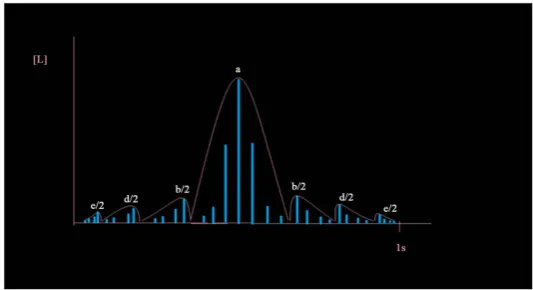
[image:4.595.241.505.383.525.2] [image:4.595.239.506.558.703.2]Our aproach is merely arithmetical; based on the application of dics. Assume that the interactions between the charge and the quantum of Action are discrete. Natural numbers are involved. They translate a set of inputs of interactions per unit of time. For that all speed values are represented by a vector with the same direction but different magnitude. Figure 1 represents grafically a set sketch of uncut, chaotic velocities. Whilst in Fig-ure 2 we represent the sum of all speeds properly ordered by mean as of the dics appli-cation.
Figure 1. Disorderly or chaotic spectrum of velocities.
Let’s start writing the dics involved
(
)
61 2 16 32 16 2 1 10 70.000.000
a= + + + + + + = (15)
(
256 128 16 8 10)
4.080b= + + + = (16)
(
128 64 8 4 10)
2.040d= + + + = (17)
(
)
31
256 128 16 8 0.408
10
e= + + + = (18)
Compute the sum of the four discrete contribution series typed above and assign
speed units 1
LT−
(
)
1 m
2187691, 26275 .
32 s
F= a b+ + +d e = (19)
Photons (light particles) travels in the vacuum at the speed of light. Therefore will compute the ratio between the sum of dics (velocities ) and the speed of light in vacuum (Appendix).
m 299.792.458
s C=
Finally write the ratio
1
137, 035999139.
C
F =α = (20)
Note that this value agrees exactly with all the significant digits, twelve significant figures, that defines the current accepted value of the inverse of the fine structure con-stant α−1.
3. Proton-electron ratio
In his book “The lightness of Being”, Franck Wilczek [4] describes in a chapter the relationship between two equations (The music of the grid. A poem in two equations). On one side the second law of Einstein
2.
E m
c
= (21)
On the other hand the Planck-Einstein-Schroedinger formula .
E=h
ν
(22)Both equations can be written as
2 .
mc h
ν = (23)
The symbol ν denotes the frequency mode of vibration. As for the mass of the proton and electron both are referred in the appendix.
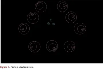
Will apply this view to the proton–electron mass ratio using dics calculation (sketched in Figure 3).
1836.153 p
e
ν
ν = (24)
Let’s apply the following series
(
128 64 8 4)
Figure 3. Proton–electron ratio.
(
)
3
1
32 16 2 1 10
b= + + + (26)
therefore
9 3 . p
e
a b
ν
ν = + (27)
3. Discussion
Since we are immersed in the theoretical approach of spacetime discreteness we went to search simple arithmetical tools. We find useful the application of a kind of series of natural numbers called dics. We have analyzed three physical topics.
Te value of the fine structure constant obtained by means of our method is the same that the current accepted value. The physical meaning is that the interaction, per unit of time between the charge of a particle and a photon isn’t unitary but complex. Despite its complexity at first sight, is capable of analyzing. The tool that we have used is able to properly order the initial complexity.
Philosophy of discreteness has guided us when we develop a practical approach to the indeterminancy principle of Heisenberg. By means of the use of dics we have seen emerge one discreteness parameter associated to the discreteness of the space, i.e. the possible range of positions of a particle.
carried by each of the three quarks, resulting nine combinations of particles with the respective color charges.
4. Conclusion
We assume a spacetime discrete. Physical variables are considered as result of the sum of discrete contributions. Such discrete contributions can be calculated with the sum of natural numbers only. Experimental physics in the atomic and subatomic realm must arrange a lot of measurements. Our approach is merely arithmetical. Some sets of series of natural numbers are involved.
References
[1] Penrose, R. (2016) The Road to Reality: A Complete Guide to the Laws of the Universe. 63. [2] Clark, A.D. (2014) Physics in Five Dimensions: Bye Bye Big Bang. 99.
[3] Mohr, P.J., et al. (2014) CODATA Recommended Values of the Fundamental Physical Constants.
[4] Wilczkek, F. (2009) The Lightness of Being. 133.
[5] L’Annunciata, M.F. (2016) Radioactivity: Introduction and History, From the Quantum to Quarks. 682.
[6] Mobilereference-2010-Tables of Universal, Electromagnetic, Atomic and Nuclear & Phy- sico-Chemical Constants.
Appendix
Table of physical constants [6]
Compton wavelength of the electron, 12
2.42631 10 m c
λ = × −
Planck constant, 34
6.62607 10 sJ
h= × −
Reduced Planck constant, 34
1.0545718 10 Js 2π
h −
= = ×
Speed of light in vacuum, : 299.792 s .458 m c
Proton mass, 27
:1.67262 10 kg p
m × −
Electron mass, 31
: 9.109383 10 kg e
m × −
Submit or recommend next manuscript to SCIRP and we will provide best service for you:
Accepting pre-submission inquiries through Email, Facebook, LinkedIn, Twitter, etc. A wide selection of journals (inclusive of 9 subjects, more than 200 journals)
Providing 24-hour high-quality service User-friendly online submission system Fair and swift peer-review system
Efficient typesetting and proofreading procedure
Display of the result of downloads and visits, as well as the number of cited articles Maximum dissemination of your research work