Collateral choice and the fundamental theorem of asset pricing

Munich Personal RePEc Archive

Collateral choice and the fundamental

theorem of asset pricing

Luis Manuel, García Muñoz

9 October 2012

Online at

https://mpra.ub.uni-muenchen.de/42451/

Collateral choice and the fundamental theorem of asset

pricing

Luis Manuel Garc´ıa Mu˜

noz ([email protected])

October 9, 2012

Abstract

In the classical quantitative finance literature it is assumed that there is a risk free rate at which hedgers can borrow and lend in the dynamic replication process of financial derivatives. In such a framework, under complete market conditions 1 and absence of arbitrage opportunities, for a given numeraire whose price cannot vanish, prices of self financing portfolios divided by the numeraire behave like a martingales under a unique martingale measure associated with the numeraire. Nevertheless, in the current market environment a high percentage of deals are collateralized due to counperparty credit risk concerns. Depending on the collateral agreement, collateral can be in the form of cash in different currencies, but also in the form of assets (bonds, shares,...). In this paper we explore how the fundamental valuation theorem and the change of numeraire tollkit is reformulated under this new framework.

1

Collateral choice implications in the replication

formula

We will assume that the derivative we want to price is written on a particular underlying whose price at timetwill be denoted bySt, that pays a continuous dividend yieldqtand

that can be repoed at a raterS

t. We will also assume that the derivative is denominated

in the same currency (L) as the underlying but, in order to reflect the most generic situation, the derivative is collateralized in an asset denominated in a different currency F.

We will use the following notation:

• St: Underlying asset price at time t.

• rSt: Repo rate of the underlying asset.

• rCt : Repo rate of the collateral asset.

• iLt: OIS (overnight index swap rate) rate in currencyL.

• iFt : OIS rate in currencyF.

• bt: Short term cross currency basis between currencies L and F (to be defined

later on).

• qt: Dividend yield (assumed continuous) of the underlying asset.

• Xt: Spot FX rate expressed in L/F

• Ct: Price of the collateral asset.

We will assume Vt to be the timet derivative’s value from the investor standpoint.

Assuming that Vt is positive, the hedger would have a positive amount Vt in cash in

currency L available as a byproduct of the dynamic replication strategy. Nevertheless Vt should be posted by the hedger to the investor in the form of the collateral asset

denominated in currencyF. Therefore the hedger will have to buy the collateral asset. By doing so, the hedger will be left with a long position in an asset denominated in currency L. Both the FX risk and the exposure to the collateral asset price changes will have to be hedged by the derivatives hedger. So that the hedger will have to enter into these transactions at a generic time step t:

• ExchangeVtin cash denominated in L for cash denominated inF in the spot FX

market.

• With the cash obtained from the FX spot transaction, the hedger will buy the

collateral asset spot and sell it forward (with maturity t+dt) through a REPO transaction. Under the REPO transaction the hedger will deliver at timet Vt

Xt in

cash denominated inF in exchange of collateral asset shares with the same value

2_.

• These shares in the collateral asset will be posted as collateral to the investor.

• At time t+dt the investor will give the collateral back (with a value of VtXCttC+tdt

measured in currency F) to the hedger, who will give it back to the REPO counterparty.

• At timet+dt the hedger will receive XVtt 1 +r

C t dt

from the REPO counterparty in cash denominated inF.

• In order to hedge the FX risk of the last amount of cash denominated in F, at

timetthe hedger should sell this amount forward (with maturityt+dt) receiving at timet+dt cash in currencyL with a value equal to the amount to be paid in currencyF (Vt

Xt 1 +r

C t dt

) multiplied by the forward FX rateXt (

1+cL t)

(1+(cF

t+bt)) seen

at timetwith maturity t+dt. We assume that forward rates cannot be inferred by the spot FX rate and the OIS rates in both currencies, so that an adjustment

needs to be made in theF rate. Notice that this adjustment represents the short term cross currency basis.

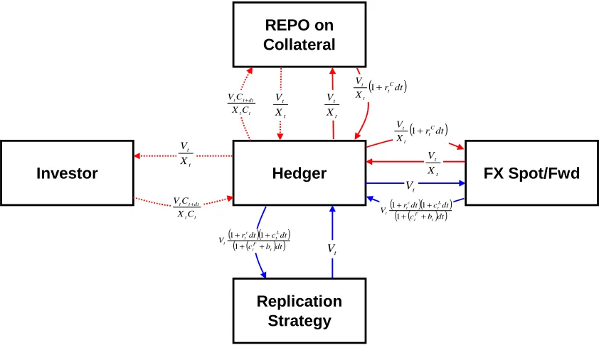
Both cash transactions (in currencies L and F) and collateral asset transactions occurring at times t and t+dt are represented in figure 1. Notice that if Vt was

negative, the trades will be right the opposite.

Hedger

Replication Strategy

FX Spot/Fwd Investor

REPO on Collateral

t

V

t

V

t t

X V

t t

X V

t t

X V

t t

X V

t t

dt t t

C X

C V +

t t

dt t t

C X

C V +

( r dt)

X

V C

t t t ₁₊

( r dt)

X

V C

t t t ₁₊

( )( )

( ) ( c bdt)

dt c dt r V

t F t

L t c t t _{+ +}

+ +

1 1 1

( )( )

( ) ( c bdt)

dt c dt r V

t F t

L t c t t _{+ +}

+ +

1 1 1

Figure 1: Continuous lines represent cash transactions whereas discontinuous ones represent asset transactions. Blue lines indicate amounts denominated in currencyL_{, whereas red ones} represent cash or asset transactions denominated in currencyF_{. Straight lines refer to initial} transactions, that take place at time t, and curved lines to final transactions taking place at time t₊dt_.

So that from ttot+dt the value of the amount deposited as collateral experiences a variation equal to:

Vt iLt +rtC−iFt −bt

dt (1)

Appart from the collateral posting mechanism and its mentioned hedges, the derivatives hedger must also hedge the delta risk associated with the underlying asset. In order to do so, the hedger

• Enters into a REPO transaction under which he receivesαtSt(assumingαtshares

of the underlying have to be purchased (or sold if negative)) in cash at timet.

• With these proceeds the hedger purchases the delta position in the underlying

asset.

• The asset is delivered to the REPO counterparty at timet.

• At time t+dt the REPO counterparty delivers both the asset position (with a

value of αtSt+dt) and the dividends paid by it in the differential time interval

• At timet+dt the hedger delivers cash to the REPO counterparty (with a value

ofαtSt 1 +rtSdt

).

Notice that if αt was negative, the trades will be right the opposite.

So that fromttot+dtthe delta hedging generates a change in the hedging portfolio equal to

αtSt+dt+αtStqtdt−αtSt 1 +rtSdt

=αtdSt+αtSt qt−rSt

dt (2)

And replication implies that the change in the value of the derivative must be equal to the change in the value of the hedging portfolio. Therefore

dVt=αtdSt+αtSt qt−rSt

dt+Vt iLt +rCt −iFt −bt

dt

Being a derivative onSand assuming any other market variable to be non stochastic, Vt must be a function of t and St. Assuming that under the real world measure St

evolves accordingly with the following stochastic differential equation:

dSt=µPtStdt+σtStdWtP

Which toghether with Itˆo’s Lemma imply

∂Vt

∂t dt+ ∂Vt

∂St

dSt+

1 2S

2

tσ2t

∂2_V

t

∂S2

t

dt=αtdSt+αtSt qt−rtS

dt+Vt iLt +rtC−iFt −bt

dt

In order to be hedged, the term in dSt must be equal in both sides of the equation,

which implies that αt= ∂V_∂St_t, so that

∂Vt

∂t +St r

S t −qt

∂Vt

∂St

+1 2S

2

tσ2t

∂2_V

t

∂S2

t

= iL_t +r_tC−iF_t −bt

Vt (3)

is the partial differential equation followed by the derivative priceVtwith boundary

condition VT =V(T, ST).

The solution to (3) is equivalent to calculating the following expected value

Vt=EQ

"

exp

−

Z T

u=t

iL_udu

VT −

Z T

u=t

exp

−

Z u

v=t

iL_vdv

Vu rCu −iFu −bu

Ft

#

(4)

Where Qis a measure under whichSt has a drift equal to rtS−qt.

In order to prove (1) we just have to apply Itˆo’s Lemma to the processVtexp

−R_ut₌₀iL udu

under Q, integrate between t and T and take the expected value conditional to the market information available at time tFt.

Notice that the second term inside the expected value of the right hand side of equation is an adjustment term to be applied to the price that we would have obtained if collateral was cash in currencyL. The reason for this adjustment is due to the exotic (non standard) collateral asset being used. The adjustment has a term that depends on the REPO OIS basis of the collateral asset, that is rC

u −iFu, and a second term due

Defininght:=iLt+rCt −iFt −btthen the solution to (3) is also equivalent to calculating

the following expected value

Vt=EQ

"

exp

−

Z T

u=t

hudu

VT

Ft

#

(5)

In order to prove (5) we just have to apply Itˆo’s Lemma to the processVtexp

−R_ut₌₀hudu

under Q, integrate between t and T and take the expected value conditional to the market information available at time tFt.

Notice that both (4) and (5) are expected values under the same measure.

2

The spot martingale measure

Assume two different derivatives on the same underlyingSwith the same payoff function g(ST) at a future timeT. The only difference with the two derivatives is that one of

them is collateralized with the underlying asset and the other with a generic collateral. The timetprices of the two derivatives will be represented byVS

t (collateralized with

the underlying) and by VC

t (collateralized with a generic collateral asset). Applying

the results obtained in the last section, the PDE’s to be solved in each case are:

∂VtS

∂t +St r

S t −qt

∂VtS

∂St

+1 2S

2

tσ2t

∂2VtS

∂S2

t

=r_tSV_tS (6)

∂VC t

∂t +St r

S t −qt

∂VC t

∂St

+ 1 2S

2

tσt2

∂2VC t

∂S2_t =htV

C

t (7)

With boundary conditions VS

T =VTC =g(ST)

So that VtS and VtC are given by the following expected values

V_tS =EQ

"

exp

−

Z T

u=t

r_uSdu

V_TS

Ft

#

(8)

V_tC =EQ

"

exp

−

Z T

u=t

hudu

V_TC

Ft

#

(9)

It is important to notice that

• Both expected values are calculated under the same pricing measureQdefined as

the measure under which the drift of the underlying isrS t −qt

• The process V

S t

exp(Rt

u=0rSudu)

is aQ-martingale.

• The process V

C t

exp(Rt

u=0hudu) is a

Q-martingale.

measure, in order to obtain martingales, each derivative should be divided by a current account that accrues at a rate equal to the short term carry rate produced by posting (or receiving) the collateral asset and hedging its risks.

In the remaining of the paper we will try to confirm this result under a different pricing measure.

3

The martingale measure associated with the

underlying asset

It is well known that the current account is not the only valid numeraire. A self financing portfolio produced by purchasing the underlying asset and reinvesting the dividends paid on it can also be used. Nevertheless, remember that in the last section it seemed that two different current accounts were used to deflate derivatives prices depending on the collateral asset being used. In this section we are about to see that a similar situation will arise when we try to use the underlying asset as numeraire.

We will first deal with VS

t , that is, the derivative collateralized with the underlying

asset.

Replication means that at a generic time intervaltthe value of the derivative must be equal to the value of the hedging portfolio

VtS =αtSt+βt

Where βt represents the value of collateral less the value of the liability created

while purchasing the delta position (or asset ifαt<0).

We define a process NS

t := StexpR_ut₌₀zudu

. NS

t will represent the numeraire

used to divide derivatives collateralized in the underlying asset. zt will be determined

by imposing the martingale condition.

If we divide every term of the replication equation by NS t

VS t

NS t

=αt

St

NS t

+ βt NS

t

Defining VS_t := VtS

NS t

VSt =αtexp

−

Z t

u=0

zudu

+βt St

exp

−

Z t

u=0

zudu

(10)

And in differential form

∂VS_t ∂t dt+

∂VS_t ∂St dSt+

1 2

∂2_VS t

∂S2

t S

2

tσ2tdt=

exp−R_ut₌₀zudu −ztαtdt+dβ_Stt −ztβ_St_tdt−_Sβt2

tdSt+

βt

Stσ

2

tdt

dβt represents the change experienced by the replicating portfolio excludingαtdSt.

Therefore, according to section 1

dβt= +αtSt qt−rSt

dt+V_tS iL_t +rC_t −iF_t −bt

Since the derivative is collateralized with the underlying asset, rtC = rtS, iFt =

iL

t, bt= 0. so that

dβt= +αtSt qt−rtS

dt+rStVtSdt

∂VSt

∂t dt+ ∂VSt

∂StdSt+

1 2

∂2_VS

t

∂S2

t

S2

tσ2tdt=

exp−R_ut₌₀zudu −ztαtdt+

αtSt(qt−rtS)+rStVtS

St dt−zt

βt

Stdt−

βt

S2

t

dSt+β_St_tσt2dt

(11) In order to be hedged, the terms in dSt in both sides of equation (11) should be

equal, so that:

βt=−S2t

∂VS_t ∂St

(12)

Which together with (10) imply

αt=

VtS

St

+St

∂VSt

∂St

(13)

Substituting (12) and (13) in (11)

∂VS_t ∂t +12

∂2_VS t

∂S2

t S

2

tσt2 =

exp−R_ut₌₀zudu −ztV

S t

St −ztSt

∂VSt

∂St + (qt−r

S t)

VS t

St + (qt−r

S t)St∂V

S t

∂St +r

S t

VS t

St +ztSt

∂VSt

∂St −σ

2

tSt∂V

S t

∂St

(14) And canceling terms

∂VS_t

∂t + (rtS−qt+σ2t)St∂V

S t

∂St +

1 2

∂2_VS t

∂S2

t S

2

tσt2 = exp

−R_ut₌₀zudu (qt−zt)V

S t

St

(15)

For VS_t to be a martingale in a measure under which the drift of St is given by

rtS−qt+σt2 (we will call this measureH),ztmust be equal toqt, so that the right hand

side of the equation equals zero. Therefore, the numeraire associated with derivatives collateralized with the underlying asset is

N_tS =Stexp

Z t

u=0

qudu

and the PDE followed by VS_t

∂VSt

∂t + (rSt −qt+σt2)St∂V

S t

∂St +

1 2

∂2VSt

∂St2 S

2

tσ2t = 0 (16)

NS

t represents the evolution of a self financing portfolio where dividends paid by

only difference now is the fact that the REPO rate associated with the underlying rSt

replaces the risk free rate rt.

The solution to (12) is

VtS

St

=EH



 VTS

STexp

RT u=tqudu

Ft



 (17)

And as already stated, H is the measure under which the drift of St is given by

rS

t −qt+σ2t

Now we handle the situation where the derivative is colateralized with a generic asset that implies a carry ofht. Remember that in section 1 we saw thatht=itL+rCt −iFt −bt.

Again, the replication equation is

V_tC =αtSt+βt

Where VtC represents the t value of the derivative collateralized in an asset with

short term carryht.

We again define a processNC

t :=Stexp

Rt

u=0zudu

. NC

t will represent the numeraire

used to divide derivatives collateralized in the assetC. zt will again be determined by

imposing the martingale condition.

If we divide every term of the replication equation by NtC

VtC

NC t

=αt

St

NC t

+ βt NC

t

Defining VeC t :=

VC t

NC t e

VtC =αtexp

−

Z t

u=0

zudu

+βt St

exp

−

Z t

u=0

zudu

(18)

And in differential form

∂VeC t

∂t dt+ ∂VeC

t

∂St dSt+

1 2

∂2VeC t

∂S2

t S

2

tσ2tdt=

exp−R_ut₌₀zudu −ztαtdt+dβ_Stt −ztβ_St_tdt−_Sβt2

tdSt+

βt

Stσ

2

tdt

dβt equals

dβt= +αtSt qt−rSt

dt+V_tS iL_t +rC_t −iF_t −bt

| {z }

ht

dt

⇓

∂VeC t

∂t dt+ ∂VeC

t

∂St dSt+

1 2

∂2VeC t

∂S2

t

S2

tσ2tdt=

exp−R_ut₌₀zudu −ztαtdt+

αtSt(qt−rSt)+htVtC

St dt−zt

βt

Stdt−

βt

S2

tdSt+

βt

Stσ

2

tdt

βt=−St2

∂VeC t

∂St

αt=

VC t

St

+St

∂VeC t

∂St

(20)

Substituting (20) in (19)

∂VeC t

∂t +

1 2

∂2_VeC t

∂St2 S

2

tσt2=

exp−R_ut₌₀zudu −ztV

C t

St −ztSt

∂VeC t

∂St + (qt−r

S t)

VC t

St + (qt−r

S t)St∂

e

VC t

∂St +ht

Vt

St +ztSt

∂VeC t

∂St −σ

2

tSt∂

e VC t ∂St (21) And canceling terms

∂VeC t

∂t + (rSt −qt+σt2)St∂

e

VC t

∂St +

1 2

∂2_VeC t

∂S2t S

2

tσt2= exp

−R_ut₌₀zudu qt−zt−rSt +ht

VC t

St

(22) ForVeC

t to be a martingale inH, under which the drift of Stis given byrSt −qt+σ2t

(same as in the case where the derivative was collateralized with the underlying asset), ztmust be equal toqt−rSt +ht, so that again the right hand side of the equation equals

zero. Therefore, the numeraire associated with derivatives collateralized with a generic collateral asset with short term carry ht is

N_tC =Stexp

Z t

u=0

qu+hu−ruS

du

and the PDE followed by VS_t

∂VeC t

∂t + (r S

t −qt+σ2t)St∂

e

VC t

∂St +

1 2

∂2VeC t

∂S2

t

S2

tσ2t = 0 (23)

NtC represents the evolution of a self financing portfolio under which we initially

invest in the underlying asset, but we continuously enter into two REPO transactions, the first withStand the second withCtas the underlying assets. Under the first REPO

transaction we deliver the position in St against cash (and pay an interest rtS on it).

This cash is converted in currencyLand delivered under the second REPO transaction against a position in Ct being received as collateral. Under this second transaction we

get a return of rC

t . Nevertheless, that in order not to incur in FX risk, we will have

to sell the amount to be received inF through this second REPO transaction forward. This will leave us with a net carry ofht−rtS. Dividends paid byStare also reinvested.

The solution of (23) is

VC t

St

=EH



 VTC

ST exp

RT

u=t(qu+hu−ruS)du

Ft   (24)

And as already stated, H is the measure under which the drift of St is given by

rS

t −qt+σ2t

To summarize, VS

t and VtC are given by the following expected values

VS t

St

=EH



 VTS

STexp

RT u=tqudu

VtC

St

=EH



 VTC

ST exp

RT

u=t(qu+hu−ruS)du

Ft  

It is important to notice that

• Both expected values are calculated under the same pricing measureHdefined as

the measure under which the drift of the underlying isrSt −qt+σt2

• The process V

S t

Stexp(R_ut₌₀qudu) is a

H-martingale.

• The process V

C t

Stexp(R_ut₌₀(qu+hu−rSu)du)

is aH-martingale.

4

The Radon-Nikodym derivative in the new

framework

Taking into account the results obtained in sections 2 and 3, lets first analyze the case of VS

t (derivative collateralized with the underlying asset)

V_tS=EQ



 VTS

expR_uT_=trS udu Ft 

=StEH



 VTS

ST exp

RT u=tqudu

Ft   So that

V_tS =EQ

       VS T

expR_uT_=trS udu

| {z }

XT Ft       

=EH

         VS T

expR_uT_=trS udu

| {z }

XT

StexpR_ut₌₀qudu

STexp

RT u=0qudu

expR_uT₌₀rS udu

expR_ut₌₀rS udu

| {z }

dQ

dH(t,T)

Ft         

So that the Radon-Nikodym derivative takes the expression of the ratio of numeraires at timettimes the inverse of the ratio of numeraires at timeT. The numeraires we are referring to are the ones used to deflate derivatives collateralized with the underlying.

In the case of VtC (derivatives collateralized with Ct), we saw in sections 2 and 3

that

VtC =EQ



 VTC

expR_uT_=thudu

Ft 

=StEH



 VTC

ST exp

RT

u=t(qu+hu−ruS)du

Ft   So that VS t =EQ

        VS T

expR_uT_=thudu

| {z }

XT Ft        

=EH           VS T

expR_uT_=thudu

| {z }

XT

StexpR_ut₌₀ qu+hu−rSu

du

STexpR_uT₌₀(qu+hu−rSu)du

expR_uT₌₀hudu

expR_ut₌₀hudu

| {z }

dQ dH(t,T)

So that the Radon-Nikodym derivative again takes the expression of the ratio of numeraires at time t _{times the inverse of the ratio of numeraires at time} T_{. The numeraires we are referring to are the ones used to deflate derivatives} collateralized with a generic collateral asset C_t.

It is very important to notice that the expression of the Radon-Nikodym derivative is the same in both cases, as we would expect with a single change of measure.

Notice also that under both Q and H, the ratio of numeraires used to deflate prices of derivatives collateralized withC_tand S_{tis given by the same expression}

N_tC,Q NS,Q

t

= N

C,H

t

NS,H

t

= exp

Z t

u=0

h_{u −}r_uSdu

5

Conclussions

• In a simplified framework under which interest rates, REPO rates and cross

currency basis spread are all non stochastic, we have seen that in order to price derivatives that are collateralized, where we could have several collateral assets available, the fundamental theorem of asset pricing needs to be reformulated.

• Contrary to the classical result, under a single pricing measure we have

different numeraires, as many as collateral assets are available.

• In order to obtain martingales, each numeraire (associated not only to a

pricing measure, but also to a collateral asset) is used to deflate derivatives collateralized in the particular collateral that defines the numeraire.

• The ratio of numeraires associated with different collateral mechanisms is

equal under any pricing measure.

• The expression of the Radon-Nikodym derivative is still related with the ratio

of numeraires times its inverse at different time instants. This expression does not depend on the particular collateral mechanism being used.

Nevertheless these conclusions have all been obtained under the assumption of non stochastic interest rates, REPO rates and spreads and in a single currency environment. All of these results should be confirmed in the most general situation.

References

[1] Vladimir Piterbarg, Funding Beyond Discounting. Collateral agreements and derivatives pricing. Risk February 2010.