An Advanced Analytical Approach for Spectral-Based Modelling of Soil Properties

(1)

International Journal of Emerging Technology and Advanced Engineering

Website: www.ijetae.com (ISSN 2250-2459, ISO 9001:2008 Certified Journal, Volume 7, Issue 3, March 2017)

90

An Advanced Analytical Approach for Spectral-Based

Modelling of Soil Properties

Nimrod Carmon

1

, Eyal Ben-Dor

2

1_{The Porter School of Environmental Studies, Tel-Aviv University} 2_{School of Geosciences, Faculty of Exact Sciences, Tel-Aviv University}

Abstract— developing accurate and robust prediction models to analyse soil attributes from spectral information has a significant importance for hyperspectral remote sensing applications. Using partial least squares for model development is a multistep process with many optional alterations. Although crucial for the result, pre-processing algorithms to be applied to a given dataset are usually selected in a non-systematic procedure that ends once the user obtains a favourable result based on a subjective impression. These results are sensitive to many aspects of model development, including grouping method, validation technique, pre-processing calculation and model statistical parameters, among others. In this study, we developed an optimal and automatic systematic procedure for model development that takes into account many possible alternatives, and includes a

novel pre-processing technique and model-validation

approach. Based on the many options available to extract a suitable model, we developed an automatic data-mining machine and parameter set to judge the results and the physical assignments used by the model, in order to extract the best model for practical remote sensing applications. An evaluation tool for correlations between spectral and modelled data is demonstrated to highlight the power of the suggested approach. The developed system, termed PARACUDA II® was tested on the legacy soil spectral library of Ben-Dor and Banin, which had been used to establish the soil chemometrics approach.

Keywords—Remote Sensing, Soil Spectroscopy, Imaging Spectroscopy, Statistical Modelling, Data Mining, Precision Agriculture, Environmental Monitoring.

I. INTRODUCTION

Remote sensing in the optical domain is advancing toward sensors with higher resolutions in the special and the spectral domains. The high (imaging) spectral resolution data, known as hyperspectral remote sensing (HSR) is playing a major role in the forthcoming spectral based applications at all spheres (hydrosphere, biosphere, geosphere, pedosphere, cryosphere and atmosphere). Among these, pedosphere has a key significance in agriculture activities and is an important factor in the food security arena (Fan et al., 2012).

As soil being the medium for plant growth, monitoring and mapping its conditions is important for maintaining sustainable agricultural activities. This can be done either by traditional methods, or as presented in the past decade, by spectroscopy and chemometrics (Mulla, 2013). Combining spectroscopy with chemometrics enables the development of various monitoring tools applicable using point spectrometers in the laboratory or the field, and using imaging spectrometers mounted on airborne and space borne platforms (Stevens et al., 2010). Recently, spectral libraries of soils are being developed worldwide to develop a big database for analyzing soil attributes remotely (Terra et al., 2015). With new missions to place a hyperspectral sensor in orbit (e.g. ENMAP (Guanter et al., 2015), SHALOM (Qian, 2016)), these soil libraries could serve as an important resource for generating thematic maps of soil attributes, providing the end user with tools for better agricultural practices. As spectroscopy from all domains plays a major role in the analysis of both chemical and physical soil parameters, HRS can extract valuable information with spatial continuity, providing an innovative and novel tool for practical applications.

(2)

International Journal of Emerging Technology and Advanced Engineering

91

As the objective here is to develop a prediction model under the most optimal conditions, careful consideration for the measurement procedures has to be made to minimize systematic and non-systematic effects from the acquired data.

Soil is a complex system that is extremely variable in physical structure and chemical composition both temporally and spatially. Soil spectroscopy, although being complex as well, can cluster several soil properties with a single measurement and a data-mining chemometric approach (Ben-Dor and Banin, 1995b). In this process, the analysis is searching for the interaction between electromagnetic radiation and active chemical groups within a chemical active group termed "chromophores" (HUNT, 1970). These chromophores' activity is due to vibration overtone modes of functional groups at the molecular level across the SWIR spectral region and to electronic transitions in atoms across the VIS-NIR spectral regions at specific wavelengths (termed "chemical chromophores"). Scattering effects based on particle size and shape distribution in the material are also active in this region and affect the whole spectrum's shape (termed "physical chromophores‖). Although there is a strong relationship between the soil chromophores as observed in the spectral domain and the chemical/physical characteristics of the material, the correlation is not straightforward. This is because the spectral data are multivariate, with many reciprocal effects (Schwartz et al., 2012). Accordingly, the extraction of quantitative information on a given soil attribute using spectral information is not a simple task, especially if it is not a chromophore attribute; a sophisticated method of finding this relationship, known as "data-mining", has to be applied. As the final goal is to use the spectral model for practical remote sensing application, it is crucial to extract the best model in a given population, rather than just finding a correlation. Many methods for applying data-mining to soil spectral information have been used and developed, from multiple linear regression (MLR) analysis (of the spectral against the chemical/physical data) through principle component analysis regression (Chang et al., 2001), partial least squares regression (PLS-R) (Zhao et al., 2015), artificial neural networks (Carmon and Ben-Dor, 2016), and random forest among others. The standard procedure for developing such models will be to divide the samples into a calibration and validation sets. The model is then developed on the spectral and chemical data of the calibration group, and is applied on the spectral data of the validation group to predict its chemical values.

The quality of the model is determined by its prediction accuracy using various statistical parameters. When a prediction model with good quality is found, it can be used to predict the chemical values of new samples with just a spectral measurement, either from point or from imaging spectrometers.

Because spectral data are affected by various components in the soil, some of which are connected to the chemical property in question and some not, applying preprocessing algorithms on the data prior to developing the model can amplify relevant spectral features and thus traditionally taking place. This notion postulate that manipulations of the original data as a part of the data mining routine might increase the final prediction accuracy. As a given dataset can be executed using several manipulation stages in a process chain, it is impossible to check many preprocessing combinations manually. Ben-Dor and Banin 1995 suggested developing a "whole-process‖ possibility chain in an automated environment to enable optimal data-mining, such that the best preprocessing combination could be selected. This concept is termed All Possibilities Approach (APA), in which all possible combinations are evaluated. Moreover, they concluded that aside from good statistical parameters and a selected processing chain, a reliable model must have solid spectral assignments for the spectral region/channels selected by the analysis. This is done by finding the important spectral ranges used by the model and examining if the selected wavelengths have a meaningful explanation based on the physical processes described earlier.

(3)

International Journal of Emerging Technology and Advanced Engineering

92

As the main goal was to develop an accurate (reliable) prediction model, based on finding the best preprocessing combination and spectral assignments, a new system was strongly sought that could fully exploit the APA idea of the PARACUDA engine but would also take into consideration the abovementioned drawbacks. Accordingly, a new version of PARCUDA, termed PARACUDA II®, was thus developed. In this new engine, not only were the above problems considered, but also the criteria for best model selection were optimized.

In this study, we developed a spectral data-mining system designed to minimize or eliminate any subjective or random considerations in the model's development, and to take into account the above drawbacks. This system, called PARACUDA II, is automatic, optimizes every

model-development step—including data preparation,

preprocessing and nLV determination—and provides a concrete validation output extracted from many partitioning of the population in use. It combines both LCV and IV methods and produces new products that contribute to a full understanding of the model's behavior and its application potential by means of supervised preprocessing. The above drawbacks are also considered in the new system, and the matter of physical explanation of the spectral assignments is addressed as well.

II. MATERIAL AND METHODS

A. Study Area and Soil Samples

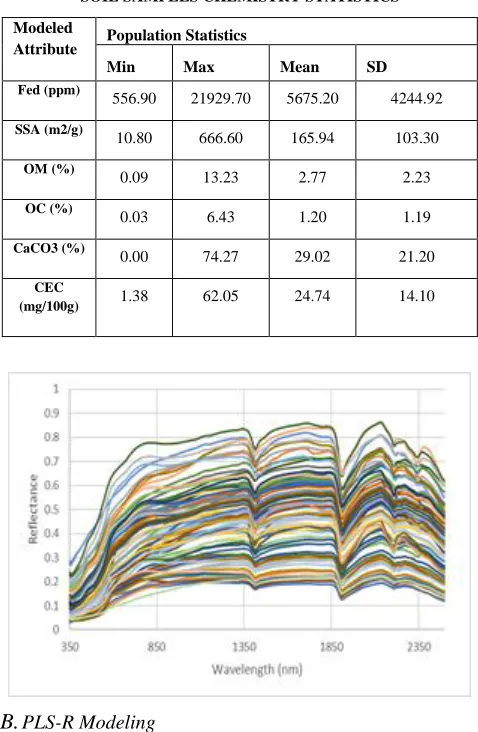
The legacy soil spectral library of Ben-Dor and Banin 1995, was used to evaluate the performance of the PARACUDA II data-mining machine. The database was composed of 91 soil samples, representing 12 Israeli soil groups, covering the semiarid to arid climate zones of Israel. The soils were collected mostly from the upper 5 cm (horizon A0) within a 1 m2 area. For this study we selected six soil attributes relevant for soil characterization: cation exchange capacity (CEC) using CNAP (Sims, 1986), free iron oxides (Fed) using DBC (Mehra and Jackson, 1960), specific surface area (SSA) using EGME (Ratner-Zohar et al., 1983), organic matter (OM) and organic carbon (OC) using dry oven drying (Ben‐ Dor and Banin, 1989), and carbonate content (CaCO3) using HCl gasometric (Ben-Dor

[image:3.612.324.563.150.516.2]

and Banin, 1990). Spectral measurements were performed using a FieldSpec Pro ASD spectrometer (Analytical Spectral Devices, Boulder CO, USA). A spectral measurement protocol combined with a standardization procedure (CSIRO and ISS) (Ben Dor et al., 2015) was used for the spectral measurements.

TABLE I

SOIL SAMPLES CHEMISTRY STATISTICS

Modeled

Attribute Population Statistics

Min Max Mean SD

Fed (ppm)

556.90 21929.70 5675.20 4244.92

SSA (m2/g)

10.80 666.60 165.94 103.30

OM (%)

0.09 13.23 2.77 2.23

OC (%)

0.03 6.43 1.20 1.19

CaCO3 (%)

0.00 74.27 29.02 21.20

CEC

(mg/100g) 1.38 62.05 24.74 14.10

B.

PLS-R Modeling

(4)

International Journal of Emerging Technology and Advanced Engineering

93

This is possible because the factors are determined under an orthogonality criteria, confirming there is no correlation between the new scores.

Several validation techniques can be used to evaluate the model‘s performance and accuracy: leverage correction (Rohe et al., 1999), leave-one-out cross validation (LCV), multifold cross validation, and internal validation (IV) (Nicolaï et al., 2007). In leave-one-out cross the entire sample population is validated in an iterative process, with one sample left out in each iteration, while the model is built on the remaining group and used to predict the sample that was left out. In each iteration, a different sample is left out and predicted by the remaining samples, until all samples have been similarly treated. In Internal validation, the entire dataset is divided into two groups: calibration and validation, which are usually partitioned into 75% and 25%, respectively, of the population examined. The model is developed on the calibration group and later projected on the validation group. This technique simulates a more real situation, in which we use one model on a set of samples, rather than using multiple models as in the LCV technique.

B. PARACUDA II®

PARACUDA II attempts to optimize all model development steps, in order to automate and standardize the modeling procedure. For this purpose we have developed three major modules, each with a specific purpose in the modeling process: (1) outlier detection and elimination; (2) preprocessing and transformations; (3) model development and validation. The whole routine for finding the best available model, and for reporting the general performance is automated, but some pre-configuration is available for the user.

1) Outlier Detection and Elimination: The system checks the data for outliers on both the chemical values and the spectra. The chemical values for the specific task is transformed into z-scores and a pre-configured threshold value to eliminate outlier is applied. The regular value is z=2, removing samples which are in the 2.5% out range of a normal distribution. For the spectral data, the system applies a principle component analysis (PCA) transformation and calculates the first two factors. Then, a 95% confidence ellipse is calculated on the two factors, and samples outside of the ellipse are considered as outlier and excluded.

2) Preprocessing and Transformations: First, the system applies box-cox transformation on the chemical data in order to achieve more normally distributed values. The spectra is than subjected to a sequence of sophisticated preprocessing calculations, based on the APA.

In this sequence, the reflectance information of the spectral data is preprocessed by employing a set of eight preprocessing algorithms: moving average, multiple scatter correction (Small, 1980), standard normal variate (Maeda et al., 1997), absorbance, continuum removal (Gomez et al., 2008), first derivative, second derivative, and final smoothing (Barnes et al., 2004). The eight algorithms are deployed in every mathematically possible combination using all possible sequences, resulting in up to 120 different combinations, as some combinations are not possible (e.g. log on a negative). After the 120 procedures have been saved, we evaluate the correlation between every spectral combination at each wavelength and the modeled attribute. The combination with the highest correlation is selected and used in further stages. The result of this sequence is a set of different transformation values for every wavelength in the data, indicating the highest covariation with the modeled properties. In this process, we exploit all manipulations for the spectral dataset rather than relying on a single, and sometimes arbitrarily selected sequence for the entire wavelength region. The final product of this step is a new dataset containing the values of different and optimal preprocessing algorithms for every wavelength separately. The correlation graphs before and after preprocessing are also saved for further evaluation.

3) Model Development and Validation: This module is meant to develop a PLS-R model on the transformed and preprocess data without overfitting. This whole module is applied iteratively, usually 256 times. First, we use a Latin hypercube sampling algorithm designed to group the data into calibration and validation sets which will represent the most variability of the data within the two groups. This is done by sub-setting the data based on the modeled attribute into 10 value ranges (bins) based on a Gaussian distribution. The system will randomly select samples from the bins in the preconfigured calibration to validation ratio. This process will be done repeatedly 100000 iterations, for each the co-variability of the two groups is calculated. The grouping resulted with the most co-variability is selected to continue in the modeling procedure.

(5)

International Journal of Emerging Technology and Advanced Engineering

94

Next, the optimal nLV is calculated by evaluating the percentage of variance explained (PCTVAR) of the modeled values for model models with between 5 and 15 factors. The second local minima is found and selected to continue to the model development procedure.

The next step is the main PLS-R model development. The system builds a model on the per-wavelength preprocessed data and the transformed chemical values with the optimal nLV and on the calibration group. The preprocessing procedure is applied on the validation group, followed by applying the PLS-R model. The prediction performance and the model itself are saved and the whole module is iterating again.

4) Population Analysis and Best Model Selection: When the iterative procedure finishes, the available data are 256 unique PLS-R models with their performance statistics. The system applies standard statistical analysis on the model population performance‘ criteria and finds the best available model from the population. The system than creates an excel file for which the R-squared from step 2.2.3 is outputted, together with the squared beta-coefficients of the best model for the best PLS-R model. The excel file also contains the predicted vs measured chemical values ready to be scatter-plotted. The resulted excel file will contain one sheet in which the best model statistics for every modeled attributed is registered, and individual sheets for every modeled attribute with the mentioned data.

III. RESULT AND DISCUSSION

The PARACUDA II system is installed on a multicore server and used 10 cores for the specific task (capable of using as many cores as available), resulting with a 5 minute operation time. All of the modeled soil properties showed remarkable results, with R-square of between 0.861 and 0.946 for applying the models on the validation set. Table 2 shows a statistical summary for all modeled attributes, which consist of the squared on the validation set, R-squared of the calibration set, RPD, RMSEP, nLV and number of valid samples used.

TABLE II

THE PARACUDA II ® PREDICTION MODELS RESULTS

Modeled Attribute

Models Statistics

R2 -test

R2_-cal _RPD _RMSEP _nLV _{# Samples}

Fed (ppm) 0.877 0.840 2.901 1041.103 7 78

SSA (m2/g) 0.911 0.881 2.113 39.736 7 82

OM (%) 0.862 0.901 2.106 0.762 8 80

OC (%) 0.946 0.937 4.360 0.170 8 79

CaCO3 (%) 0.941 0.946 3.491 5.760 9 83

CEC (mg/100g)

0.942 0.928 2.511 5.383 9 81

A. Individual Properties

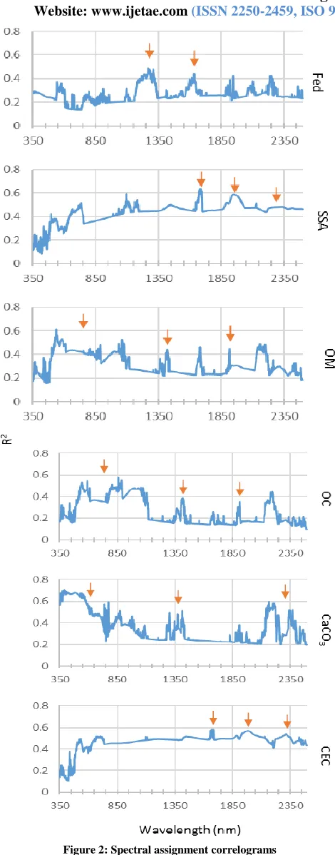
One of the important stages in developing spectral prediction models is to check whether the wavelengths selected by the models are fully spectrally assigned to the property in question or perhaps correlated with noise. The spectral assignment procedure is hence a crucial stage in model validation and conformation. To that end, PARACUDA II was programed to provide a correlogram spectrum in which the wavelengths weights for each model are plotted. The following session provides a discussion on each soil property with the statists accuracy obtained by the PARACUDA II with statistics obtained for the same population 25 years ago by Ben-Dor and Banin 1995 using the first attempt to use chemometric approach for soil using MLR. Also provided is a discussion on the best wavelengths and possible physical assignment for every selected model.

(6)

International Journal of Emerging Technology and Advanced Engineering

[image:6.612.49.284.116.715.2]

95

Figure 2: Spectral assignment correlograms

Accordingly Ben-Dor 1992, found that Fed (direct chromophore) has correlation with TiO2 (R=0.72) which is also direct chromophore in the VIS region, with clay minerals that are active in the SWIR (R with Smectite - 0.57 and with Al203 - 0.81) that all are active in the SWIR regions. The assignment at around 1700 nm may be due to the correlation of Fed with aggregate size distribution (R= 0.51). The above correlations provide explanation to the model assignments found by PARACUDA II and demonstrate the idea that every model has to have a significant spectral assignment. The Fed modeling of the same population as done by Ben Dor and Banin 1995 using the MLR approach which was the optimal way to spectral modeling the soil properties at that time yielded R2=0.59, SEP = 2873 ppm and RPD of 1.2. Most of the assignment found then were from the VIS-NIR region. From the results obtained in this study, it is apparent that the PARACUDA II were able to yield better results with the same exact population 25 years after and demonstrates the strength of this approach.

2) SSA: Modelling of the specific surface area (SSA) shows R2 = 0.91, SEP = 39.74 m2/g and RPD of 2.11. In general the SSA will normally be assigned to the clay minerals (Smectite) that active at around 2200 nm, where it can be also recognized in the VIS-NIR region as it correlates to organic matter (R=0.51), Fed (R=0.61), TiO2 (R=0.62) Mn

(R= 0.732) and more heavy metals that all are active in the VIS-NIR and hence be indirect chromophores for the SSA property. The spectral assignment graph shows also correlation around 1500 nm and the 1900 nm that can be assigned to OH of the adsorbed water molecules. The modeling of Ben Dor and Banin from 1995 using the MLR approach, provided R2=0.69 with SEP =50.2 and RPD = 1.3. The PARCUDA II performances showed a significant improvement is all these parameters demonstrated the power of it relative to the traditional first approach.

(7)

International Journal of Emerging Technology and Advanced Engineering

96

Most of the assignment found then were from the VIS-NIR region. As apparent, the PARACUDA II yielded better results.

4) OC: Modeling the Organic Carbone (OC) yielded higher accuracy than the OM although the relationship between them is very high (R = 0.94). The modeling provided R2=0.95, SEP of 0.17% and RPD of 4.4 (see Table II). The spectral assignment graph shows high similarities with the OM across the entire spectral region. The better accuracy obtained for the OC is due to the fact that in the modeling of OM, also other components might be spectrally active and reduce the OM accuracy than the OC. Apparently in Ben-Dor and Banin 1995 no modeling for OC was given.

5) CaCO3: Modeling of the calcium carbonate yielded

R2=0.94, SEP= 5.76% and RPD =3.5 (see Table II). The assignments were mostly observed at SWIR-2 and around the VIS-NIR region that are assigned directly to CO3 and to

other elements correlate to CaCO3 and characterize with

direct chromophore. In the VIS region heavy metals are highly correlated to CaCO3 with Ti02 (R=0.53), CO (R=0.69) and others which explain why the CaCO3 has

correlation in the VIS-NIR region. The strong assignment at around 2300 nm is related to the CO3 overtone where the

other SWIR region may probably explain by the Silt content (R=0.57) that is reached with K (R=0.49) and Illitic minerals. The modeling of Ben-Dor and Banin from 1995 using the MLR approach yielded R2=0.67, SEP = 11.6 and RPD =1.5. It is apparent that the PARACUDA II were able also here to yield better results with the same population.

6) CEC: The CEC is similar to SSA although less informative. It is apparent that CEC is indirectly correlated with SSA (R=0.73) based on to the clay mineral spectral assignments. The R2 Ben-Dor and Banin 1995 found for the CEC content for this exact population was high (R2=0.64) but no as high as here (R2=0.94) demonstrating the power of the PARACUDA II.

IV. DISCUSSION

The better accuracy obtained by the PARCIDA II as compare to a traditional method (MLR) points out that in a given population it is unlikely that there is only one model which is usually the first good one found by the user. PARACUDA II helps to check other possible models which is not possible to get manually. Although it is likely that we still did not contain whole possible models, it is sure that many hidden model are now exposed. Applying a by-wavelength spectral preprocessing extracts more correlated data to be modeled.

The correlogram provided by the system is a very important validation and understanding tool. Besides of providing the possibility to track after the physical basis of the model it monitor the indirect correlation obtained between properties (chromophoric and non-chromophoric). This is why the correlogram is highly correlated in CEC, OM and OC. In general taking into account the final results and the efficient way to get a reliable model to every constituent is promising.

V. CONCLUSION

The prediction results together with spectral assignment explanation may provide a dipper understanding on the validity and robustness of the model. Apart from providing a validation tool for the specific task, this data can be used in future project for optimal band selection when developing new sensors. To that end it is very important that a correlation matrix between all chemical attributes will be studied to explain spectral feature the PARACUDA II extract for the best model (out of many checked). It is apparent that PARACUDA II bring a highly elaborated and robust modeling technique to a basic user with powerful automated nature. The possibility to evaluate this amount of models on a manual fashion is impossible and would take weeks for a single operator using standard modeling software.

Acknowledgments

This work was supported in part by the "Survey of Israel" under research grant 2016-2017 and by "Transportation Innovation" institute at "The Porter School of Environmental Studies" in Tel-Aviv University.

REFERENCES

[1] Barnes, R. J., M. S. Dhanoa, and S. J. Lister. ―Letter: Correction to the Description of Standard Normal Variate (SNV) and De-Trend (DT) Ransformations in <I>Practical Spectroscopy with Applications in Food and Everage Analysis–2nd Edition</I>.‖ Journal of Near Infrared Spectroscopy 1.3 (2004): 185–186. www.impublications.com. Web.

[2] Ben Dor, Eyal, Cindy Ong, and Ian C. Lau. ―Reflectance Measurements of Soils in the Laboratory: Standards and Protocols.‖ Geoderma 245–246 (2015): 112–124. ScienceDirect. Web. [3] Ben-Dor, E. ―Quantitative Remote Sensing of Soil Properties.‖ Ed.

BT - Advances in Agronomy. Vol. 75. Academic Press, 2002. 173– 243. ScienceDirect. Web. 19 Jan. 2017.

(8)

International Journal of Emerging Technology and Advanced Engineering

97

[5] Ben-Dor, E., and A. Banin. ―Near-Infrared Analysis as a Rapid

Method to Simultaneously Evaluate Several Soil Properties.‖ Soil Science Society of America Journal 59.2 (1995): 364–372. dl.sciencesocieties.org. Web.

[6] ---. ―Near-Infrared Analysis as a Rapid Method to Simultaneously Evaluate Several Soil Properties.‖ Soil Science Society of America Journal 59.2 (1995): 364. CrossRef. Web.

[7] ---. ―Near-Infrared Reflectance Analysis of Carbonate Concentration in Soils.‖ Applied Spectroscopy 44.6 (1990): 1064–1069. Print. [8] Ben-Dor, E., J. R. Irons, and G. F. Epema. ―Soil Reflettante.‖ Man

Remote Sens Remote Sens Earth Science 3 (1999): 111. Print. [9] Carmon, N., and E. Ben-Dor. ―Rapid Assessment of Dynamic

Friction Coefficient of Asphalt Pavement Using Reflectance Spectroscopy.‖ IEEE Geoscience and Remote Sensing Letters 13.5 (2016): 721–724. IEEE Xplore. Web.

[10] Chang, Cheng-Wen et al. ―Near-Infrared Reflectance Spectroscopy– Principal Components Regression Analyses of Soil Properties.‖ Soil Science Society of America Journal 65.2 (2001): 480. CrossRef. Web.

[11] Fan, Mingsheng et al. ―Improving Crop Productivity and Resource Use Efficiency to Ensure Food Security and Environmental Quality in China.‖ Journal of Experimental Botany 63.1 (2012): 13–24. academic.oup.com. Web.

[12] Gomez, Cécile, Philippe Lagacherie, and Guillaume Coulouma. ―Continuum Removal versus PLSR Method for Clay and Calcium Carbonate Content Estimation from Laboratory and Airborne Hyperspectral Measurements.‖ Geoderma 148.2 (2008): 141–148. ScienceDirect. Web.

[13] Guanter, Luis et al. ―The EnMAP Spaceborne Imaging Spectroscopy Mission for Earth Observation.‖ Remote Sensing 7.7 (2015): 8830– 8857. www.mdpi.com. Web.

[14] HUNT, G. R. ―Visible and near-Infrared Spectra of Minerals and Rocks : I Silicate Minerals.‖ Modern Geology 1 (1970): 283–300. Print.

[15] Maeda, Hisashi et al. ―Near Infrared Spectroscopy and Chemometrics Studies of Temperature-Dependent Spectral Variations of Water: Relationship between Spectral Changes and Hydrogen Bonds.‖ Journal of Near Infrared Spectroscopy 3.4 (1997): 191–201. www.impublications.com. Web.

[16] Mehra, O. P., and M. L. Jackson. ―Iron Oxide Removalfrom Soilsand Clays by a Dithionite-Citrate System with Sodium Bicarbonate Buffer.‖ 7th Conference on Clays and Clay Minerals. N.p., 1960. 317–327. Print.

[17] Minasny, Budiman, and Alex B. McBratney. ―A Conditioned Latin Hypercube Method for Sampling in the Presence of Ancillary Information.‖ Computers & Geosciences 32.9 (2006): 1378–1388. ScienceDirect. Web.

[18] Mulla, David J. ―Twenty Five Years of Remote Sensing in Precision Agriculture: Key Advances and Remaining Knowledge Gaps.‖ Biosystems Engineering 114.4 (2013): 358–371. ScienceDirect. Web. Special Issue: Sensing Technologies for Sustainable Agriculture.

[19] Nicolaï, Bart M. et al. ―Nondestructive Measurement of Fruit and Vegetable Quality by Means of NIR Spectroscopy: A Review.‖ Postharvest Biology and Technology 46.2 (2007): 99–118. ScienceDirect. Web.

[20] Qian, Shen-En. Optical Payloads for Space Missions. John Wiley & Sons, 2016. Print.

[21] Ratner-Zohar, Yael, A. Banin, and Y. Chen. ―Oven Drying as a Pretreatment for Surface-Area Determinations of Soils and Clays.‖ Soil Science Society of America Journal 47.5 (1983): 1056–1058. dl.sciencesocieties.org. Web.

[22] Rohe, Thomas et al. ―Near Infrared (NIR) Spectroscopy for in-Line Monitoring of Polymer Extrusion Processes.‖ Talanta 50.2 (1999): 283–290. ScienceDirect. Web.

[23] Rossel, R. A. Viscarra et al. ―A Global Spectral Library to Characterize the World‘s Soil.‖ ResearchGate (2016): n. pag. www.researchgate.net. Web. 14 Aug. 2016.

[24] Schwartz, Guy, Eyal Ben-Dor, and Gil Eshel. ―Quantitative Analysis of Total Petroleum Hydrocarbons in Soils: Comparison between Reflectance Spectroscopy and Solvent Extraction by 3 Certified Laboratories.‖ Applied and Environmental Soil Science 2012 (2012): e751956. www.hindawi.com. Web.

[25] Sims, J. Thomas. ―Soil pH Effects on the Distribution and Plant Availability of Manganese, Copper, and Zinc.‖ Soil Science Society of America Journal 50.2 (1986): 367–373. dl.sciencesocieties.org. Web.

[26] Small, N. J. H. ―Marginal Skewness and Kurtosis in Testing Multivariate Normality.‖ Journal of the Royal Statistical Society. Series C (Applied Statistics) 29.1 (1980): 85–87. JSTOR. Web. [27] Stevens, Antoine, Bas van Wesemael, et al. ―Laboratory, Field and

Airborne Spectroscopy for Monitoring Organic Carbon Content in Agricultural Soils.‖ Geoderma 144.1–2 (2008): 395–404. ScienceDirect. Web. Antarctic Soils and Soil Forming Processes in a Changing Environment.

[28] Stevens, Antoine, Thomas Udelhoven, et al. ―Measuring Soil Organic Carbon in Croplands at Regional Scale Using Airborne Imaging Spectroscopy.‖ Geoderma 158.1–2 (2010): 32–45. ScienceDirect. Web. Diffuse Reflectance Spectroscopy in Soil Science and Land Resource Assessment.

[29] Terra, Fabrício S., José A. M. Demattê, and Raphael A. Viscarra Rossel. ―Spectral Libraries for Quantitative Analyses of Tropical Brazilian Soils: Comparing vis–NIR and Mid-IR Reflectance Data.‖ Geoderma 255–256 (2015): 81–93. ScienceDirect. Web.

[30] Wold, Svante, Michael Sjöström, and Lennart Eriksson. ―PLS-Regression: A Basic Tool of Chemometrics.‖ Chemometrics and Intelligent Laboratory Systems 58.2 (2001): 109–130. ScienceDirect. Web.