How to cite this paper: Murase, K., Nanjo, T., Sugawara, Y., Hirata, M. and Mochizuki, T. (2015) Usefulness of an Anisotrop-ic Diffusion Method in Cerebral CT Perfusion Study Using Multi-Detector Row CT. Open Journal of MedAnisotrop-ical Imaging, 5, 106- 116. http://dx.doi.org/10.4236/ojmi.2015.53015
Teruhito Mochizuki
1Department of Medical Physics and Engineering, Division of Medical Technology and Science, Faculty of
Health Science, Graduate School of Medicine, Osaka University, Osaka, Japan
2Department of Radiology, Graduate School of Medicine, Ehime University, Ehime, Japan
Email: *[email protected]
Received 21 July 2015; accepted 29 August 2015; published 2 September 2015
Copyright © 2015 by authors and Scientific Research Publishing Inc.
This work is licensed under the Creative Commons Attribution International License (CC BY). http://creativecommons.org/licenses/by/4.0/
Abstract
Purpose: To present an application of the anisotropic diffusion (AD) method to improve the accu-racy of the functional images of perfusion parameters such as cerebral blood flow (CBF), cerebral blood volume (CBV) and mean transit time (MTT) generated from cerebral CT perfusion studies using multi-detector row CT (MDCT). Materials and Methods: Continuous scans (1 sec/rotation ×60 sec) consisting of four 5-mm-thick contiguous slices were acquired after an intravenous injec-tion of iodinated contrast material in 6 patients with cerebrovascular disease using an MDCT scanner with a tube voltage of 80 kVp and a tube current of 200 mA. New image data were gener-ated by thinning out the above original images at an interval of 2 sec or 3 sec. The thinned-out im-ages were then interpolated by linear interpolation to generate the same number of imim-ages as originally acquired. The CBF, CBV and MTT images were generated using deconvolution analysis based on singular value decomposition. Results: When using the AD method, the correlation coef-ficient between the MTT values obtained from the original and thinned-out images was signifi-cantly improved. Furthermore, the coefficients of variation of the CBF, CBV and MTT values in the white matter significantly decreased as compared to not using the AD method. Conclusion: Our results suggest that the AD method is useful for improving the accuracy of the functional images of perfusion parameters and for reducing radiation exposure in cerebral CT perfusion studies using MDCT.
Keywords
Anisotropic Diffusion Method, Cerebral CT Perfusion Study, Multi-Detector Row CT, Radiation *
Exposure
1. Introduction
Cerebral perfusion studies using X-ray computed tomography (CT) have become increasingly important for management and/or prognostic prediction of stroke patients [1]. CT perfusion studies can be performed with the dynamic acquisition of sequential CT sections in cine mode during the intravenous administration of iodinated contrast material using a standard spiral CT scanner or multi-detector row CT (MDCT) [2] [3]. However, radia-tion exposure during CT perfusion study is a serious problem and is one of the hurdles preventing this procedure from becoming widespread [4]. One of the methods for reducing the radiation exposure is to reduce the X-ray tube current of CT and/or to make the time for X-ray exposure as short as possible. Previously, we proposed a method for reducing the radiation dose in cerebral CT perfusion studies by using a variable scan schedule [5]. However, reducing the X-ray tube current and/or shortening the X-ray exposure time can cause an increase of the statistical noise in the dynamic images, leading to deterioration of the accuracy of the perfusion parameters calculated from the dynamic images [5].
To reduce image noise, various filtering techniques have been devised [6]. In linear spatial filtering such as Gaussian filtering, the content of a pixel is given the value of the weighted average of its immediate neighbors. This filtering reduces the amplitude of noise fluctuations, but also degrades sharp details such as lines or edges, and the resulting images appear blurred and diffused [6]. This undesirable effect can be reduced or avoided by designing nonlinear filters, the most common technique being median filtering. With median filtering, the value of an output pixel is determined by the median of the neighboring pixels [7]. This filtering retains edges, but re-sults in a loss of resolution by suppressing fine details. Perona and Malik [8] developed a multiscale smoothing and edge detection scheme based on anisotropic diffusion (AD), which is a new concept for image processing. Their AD method overcomes the major drawbacks of conventional spatial filtering, and significantly improves image quality while preserving spatial resolution [8]-[10]. The purpose of this study was to present an applica-tion of the AD method to cerebral CT perfusion studies using MDCT for improving the accuracy of perfusion parameters and to investigate its usefulness and feasibility in reducing radiation exposure.
2. Materials and Methods
2.1. Data AcquisitionSix patients with cerebrovascular disease [3 males and 3 females; age, 69.0 ± 5.7 (mean±standard deviation) years] participated in this study. The details of the patients are described in [5]. Informed consent was obtained from each patient after a detailed explanation of the purpose of the study and scanning procedures. Following a standard protocol for CT perfusion study, continuous (cine) scans (1 sec/rotation ×60 sec) consisting of four 5-mm-thick contiguous slices were acquired after an injection of iodinated contrast material (300 mgI/mL, 30 - 40 mL) into a peripheral vein through a 20-gauge catheter with an injection velocity of 4 mL/sec, using an MDCT scanner (LightSpeed QX/i, GE Medical Systems, Tokyo, Japan) with a tube voltage of 80 kVp and a tube current of 200 mA. The 60 images obtained in each of the four slices were defined as “original images”. New image data were generated by thinning out the original images at an interval of 2 sec or 3 sec. The thinned- out images were then interpolated by linear interpolation to generate the same number of images as originally acquired. We call the images generated by thinning out the original images at an interval of 2 sec and linear in-terpolation “2-sec-interpolated images”. Similarly, we call the images generated by thinning out the original images at an interval of 3 sec and linear interpolation “3-sec-interpolated images”.
2.2. Anisotropic Diffusion (AD) Method
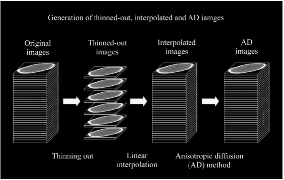
The interpolated images were processed by the AD method. We call the 2-sec- and 3-sec-interpolated images processed by the AD method “2-sec-AD images” and “3-sec-AD images”, respectively.Figure 1 illustrates how the thinned-out, interpolated and AD images were generated from the original images.
Figure 1.Illustration of generating the thinned-out, interpolated and aniso-tropic diffusion (AD) images from original images. The thinned-out images were generated by thinning out the original images at an interval of 2 sec or 3 sec. The thinned-out images were then interpolated by linear interpolation to generate the same number of images as originally acquired (interpolated im-ages). We call the images generated by thinning out the original images at an interval of 2 sec and linear interpolation “2-sec-interpolated images”. Simi-larly, we call the images generated by thinning out the original images at an interval of 3 sec and linear interpolation “3-sec-interpolated images”. The in-terpolated images were processed by the AD method to generate the AD im-ages. We call the 2-sec- and 3-sec-interpolated images processed by the AD
method “2-sec-AD images” and “3-sec-AD images”, respectively.
by selecting locally adaptive diffusion strengths [8]-[10]. This process can be formulated as follows, assuming no sinks or sources [8]-[10]:
( )
,(
( )
( )
)
div , ,
I x t
C x t I x t
t
∂
= ⋅∇
∂ (1)
where ∇I x t
( )
, represents the magnitude of the image gradient at x. The variable t is the process-ordering pa-rameter; in the discrete implementation it is used to enumerate iteration steps [9]. C x t( )
, represents a diffu-sion function which controls the diffudiffu-sion strength. In this study, we used the following function given by Tu-key’s Biweight as C x t( )
, [11]:( )
( )
( )
2 2 , 1 , , 0 otherwiseΙ x t
I x t
C x t σ σ
∇ − ∇ ≤ = (2)
where σ is the scale parameter. In this study, we chose a value for the scale parameter σ so that it begins rejecting outliers at the “robust scale” σe [11]. The “robust scale” σe is given by [12]
( )
1.4826 MAD
e I
σ = ⋅ ∇ (3)
where MAD denotes the median absolute deviation and the constant is derived from the fact that the MAD of a zero-mean normal distribution with unit variance is 0.6745 = 1/1.4826.
Numerical implementation of Equation (1) was performed in a standard manner by substituting partial deri- vatives with the appropriate discrete sample differences of the image data. Details of the discretization of Equa-tion (1) can be found in Perona and Malik [8] and Fischl and Schwarz [13].
2.3. Generation of CBF, CBV and MTT Images
concentra-tion of the contrast agent in the volume of interest (VOI) [CVOI
( )
t ] is given by [15]( )
( ) (
)
VOI CBF 0 AIF d
t
C t =
∫
C τ R t−τ τ (4)In Equation (4), CAIF
( )
t is the time-dependent concentration of the contrast agent in a feeding artery. R t( )
is the residue function which is the relative amount of contrast agent in the VOI in an idealized perfusion expe-riment, where a unit area bolus is instantaneously injected [R
( )
0 =1] and subsequently washed out by perfusion [R( )
∞ =0]. It is known from Equation (4) that the initial height of the deconvolved time-concentration curve equals the cerebral blood flow (CBF). In this study, the CBF value was obtained from the maximum value of the deconvolved time-concentration curve. There are several possible approaches to calculating CBF from Equation (4) by deconvolution [16] [17]. In this study, we adopted an algebraic approach based on singular value decompo-sition (SVD) [16] [17], which was robust against statistical noise. The details of this approach have been de-scribed elsewhere [16] [17]. When using SVD in deconvolution analysis, the elements in the diagonal matrix obtained by SVD were set to zero when they were smaller than the threshold value given beforehand. In this study, the threshold value was taken as 0.2 [16] [17]. We generated the CBF images by applying this approach pixel by pixel. The arterial input function [CAIF( )
t ] was obtained from the middle cerebral artery using fuzzyc-means clustering [18].
The cerebral blood volume (CBV) was given by the following formula:
( )
( )
VOI 0 AIF 0 d CBV d C C τ τ τ τ ∞ ∞ =∫
∫
(5)From the central volume principle [14], the mean transit time (MTT) was obtained by the equation: CBV
MTT CBF
= (6)
The CBV and MTT images were generated by applying Equations (5) and (6) pixel by pixel, respectively.
2.4. Evaluation and Statistical Analysis
To quantitatively evaluate the usefulness of the AD method, we drew 5 regions of interest (ROIs) of approx-imately 300 mm2 on each slice level of the CBF, CBV and MTT images, i.e., a total of 20 ROIs. The positions of the ROIs were as follows: 1) white matter of right frontal lobe, 2) white matter of right temporal lobe, 3) white matter of left frontal lobe, 4) white matter of left temporal lobe and 5) basal ganglia. When drawing ROIs, large blood vessels were carefully excluded. We calculated the correlation coefficients between the perfusion parameter values obtained from the original and AD images for the above 20 ROIs using linear regression anal-ysis. For comparison, we also calculated the correlation coefficients between the perfusion parameter values ob-tained from the original and interpolated images. Bland-Altman plots [19] were also generated. Furthermore, the mean and standard deviation (SD) of the perfusion parameter values in the white matter were obtained, and the coefficients of variation (CVs) were calculated from SD/mean.
The statistical comparisons of the correlation coefficients and CV values were performed using the paired Student t test. P values less than 0.05 were considered to be significant in all statistical analyses.
3. Results
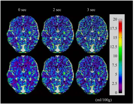
Figure 2 shows typical examples of the CBF images generated from original, interpolated and AD images. The upper left, middle and right panels show the CBF images generated from the original, 2-sec-interpolated and 3-sec-interpolated images, respectively, while the lower left, middle and right panels show those generated from the original images processed by the AD method, 2-sec-AD and 3-sec-AD images, respectively.Figure 3 and
Figure 4show the cases of CBV and MTT, respectively. As shown inFigures 2-4, the statistical noise was re-duced by using the AD method while preserving spatial resolution for all cases.
Figure 2.Typical examples of the cerebral blood flow (CBF) images generated from the original, interpolated and AD images. The upper left, middle and right panels show the CBF images generated from the origi-nal, 2-sec-interpolated and 3-sec-interpolated images, respectively, while the lower left, middle and right panels show those generated from the original images processed by the AD method, 2-sec-AD and 3-sec-AD images, respectively.
Figure 3.Typical examples of the cerebral blood volume (CBV) images
[image:5.595.182.446.84.288.2]generated from the original, interpolated and AD images. The upper left, middle and right panels show the CBV images generated from the orig-inal, 2-sec-interpolated and 3-sec-interpolated images, respectively, while the lower left, middle and right panels show those generated from the original images processed by the AD method, 2-sec-AD and 3-sec-AD images, respectively.
[image:5.595.182.446.376.580.2]Figure 4. Typical examples of the mean transit time (MTT) images generated from the original, interpolated and AD images. The upper left, middle and right panels show the MTT images generated from the orig-inal, 2-sec-interpolated and 3-sec-interpolated images, respectively, while the lower left, middle and right panels show those generated from the original images processed by the AD method, 2-sec-AD and 3-sec-AD images, respectively.
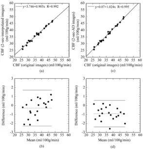
Figure 5.(a) and (b) show typical examples of the correlation and Bland-Altman plot between the
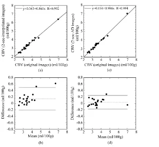
[image:6.595.182.446.84.289.2] [image:6.595.167.462.376.683.2]Figure 6.(a) and (b) show typical examples of the correlation and Bland-Altman plot between the CBV values obtained from the original and 2-sec-interpolated images, respectively, while (c) and (d) show those between the CBV values obtained from the original and 2-sec-AD images, respectively.
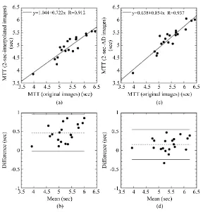
AD images, respectively. The error bar represents the SD for 6 patients. As shown inFigure 8, the correlation coefficients deteriorated with increasing thinning-out interval for all perfusion parameters. The deterioration was the largest in MTT. The correlation coefficient for MTT was significantly improved by using the AD method for both cases with thinning-out intervals of 2 sec and 3 sec.
Figure 9 shows the CV values of CBF (a), CBV (b) and MTT (c) in the white matter obtained from the im-ages with various thinning-out intervals. “0 sec”, “2 sec” and “3 sec” represent the CV values obtained from the original images or original images processed by the AD method, 2-sec-interpolated or 2-sec-AD images and 3-sec-interpolated or 3-sec-AD images, respectively. The closed and open bar graphs show the CV values ob-tained from the images without and with processing by the AD method, respectively. The error bar represents the SD for 6 patients. As shown inFigure 9, the CV values obtained from the images processed by the AD me-thod were significantly lower than those obtained without using the AD meme-thod for all cases.
4. Discussion
We previously presented an application of the AD method to improving the accuracy of the CBF images gener-ated from dynamic susceptibility contrast-enhanced magnetic resonance imaging (DSC-MRI) [10]. In the above study, we investigated the usefulness of the AD method using computer simulations and clinical data in com-parison with the median and Gaussian filters [10]. Although the median and Gaussian filters also reduced image noise, the accuracy of the CBF values considerably deteriorated. On the other hand, the AD method was capable of reducing the image noise while preserving the quantitative accuracy of the CBF images. We concluded that the AD method will make the CBF images generated from DSC-MRI more reliable [10]. In this study, we pre-sented an application of the AD method to cerebral CT perfusion studies. The present study also demonstrated that the AD method was useful for improving the accuracy of the functional images of CBF, CBV and MTT generated from cerebral CT perfusion studies.
[image:7.595.173.499.80.382.2]Figure 7. (a) and (b) show typical examples of the correlation and Bland-Altman plot between the MTT values obtained from the original and 2-sec-interpolated images, respectively, while (c) and (d) show those between the MTT values obtained from the original and 2-sec-AD images, respectively.
Figure 8.Correlation coefficients between the perfusion parameter values obtained from the original and interpolated or AD
images in 6 patients. (a), (b) and (c) show the cases of CBF, CBV and MTT, respectively. The closed and open bar graphs represent the data obtained from the images without and with processing by the AD method, respectively. “2 sec” and “3 sec” represent the data obtained from the 2-sec-interpolated (closed) or 2-sec-AD images (open) and 3-sec-interpolated (closed) or 3-sec-AD images (open), respectively. The error bar represents the standard deviation (SD) for 6 patients. *P < 0.05.
[image:8.595.91.538.421.581.2]ages with various thinning-out intervals. “0 sec” represents the data obtained from the original images or original images processed by the AD method, while “2 sec” and “3 sec” represent the data obtained from the 2-sec-interpolated or 2-sec-AD images and 3-sec-interpolated or 3-sec-AD images, respectively. The closed and open bar graphs show the data obtained from the images without and with processing by the AD method, respectively. The error bar represents the SD for 6 patients.
*
P < 0.05.
fixed for acquisitions taken under similar conditions. However, such a procedure is very time-consuming and is not suitable in a clinical setting. In this study, this parameter was automatically selected from robust statistics to estimate the “robust scale” of the image [12]. The “robust scale” is given by Equation (3). Since the scale para-meter selected from the “robust scale” worked very well, we believe that this selection can also be applied to cerebral CT perfusion studies.
A second parameter that must be selected is the number of filter operations. The iterated filter operations re-sulted in a sequence of diffused images, and impressive improvements were obtained from three to five itera-tions (data not shown). These findings are very similar to those reported by Gerig et al. [9] and our previous re-sults [10]. Therefore, all the results shown here were obtained by fixing the number of filter operations at five.
As previously described, one of the methods for reducing the radiation exposure in cerebral CT perfusion stu-dies is to reduce the X-ray tube current [4] and/or to shorten the X-ray exposure time [5]. Previously, we pro-posed a method for reducing the radiation dose by using a variable scan schedule [5]. Our previous study [5]
demonstrated that to keep the correlation coefficients of all perfusion parameters greater than 0.9, the estimated radiation dose could be reduced to 58.3% with a scan schedule of 10 continuous images and thinning-out inter-val of 2 sec. The radiation exposure decreased with increasing thinning-out interinter-val. Taking the radiation expo-sure in the case when using original images as 100%, the radiation dose became 50% and 33% when using thin-ning-out intervals of 2 sec and 3 sec, respectively. Although increasing the thinthin-ning-out interval is useful for re-ducing the radiation dose, it will cause an increase of image noise, leading to deterioration of the accuracy of perfusion parameters. As shown inFigure 8, the correlation coefficients between the perfusion parameters ob-tained from the original and interpolated images deteriorated with increasing thinning-out interval. However, the quality of the functional images of CBF, CBV and MTT was visually improved by using the AD method as shown in Figures 2-4. Furthermore, as shown inFigure 9, the CV values of the perfusion parameters in the white matter were significantly improved by using the AD method. These results suggest that the AD method is useful for reducing radiation exposure by decreasing the X-ray tube current [4] and/or by shortening the X-ray exposure time [5].
Kikuchi et al. [20] reported the usefulness of MTT images for evaluation of the extent of cerebral perfusion reserve impairment in patients with occlusive cerebrovascular disease. Therefore, it is desirable to maintain the reliability of MTT values similar to those of CBF and CBV values. The AD method appears to be useful in this respect, because the correlation coefficient between the MTT values obtained from the original and thinned-out images was significantly improved by using the AD method as shown inFigure 8.
[image:9.595.89.540.78.242.2]Furthermore, the perfusion parameters in the gray matter tended to be contaminated by those in the large blood vessels as shown inFigures 2-4.
The present study had some limitations. The number of patients was small, and they had little variation in their cerebral hemodynamic patterns. Few prominent abnormalities of cerebral perfusion parameters were found in these patients. An additional study using more patients with various types of ischemic disease or diseases of the systemic circulation is recommended to enhance the reliability of the present study.
5. Conclusion
Our results suggest that the AD method is useful for improving the accuracy of the functional images of cerebral perfusion parameters and for reducing radiation exposure in cerebral CT perfusion studies using MDCT.
Acknowledgements
This work was supported by a Grant-in-Aid for Scientific Research (Grant Number: 25282131) from the Japan Society for the Promotion of Science (JSPS).
Declaration of Interest
The authors report no conflicts of interest.
References
[1] Wintermark, M., Reichhart, M., Thiran, J.P., Maeder, P., Chalaron, M., Schnyder, P., Bougousslavsky, J. and Meuli, R. (2002) Prognostic Accuracy of Cerebral Blood Flow Measurement by Perfusion Computed Tomography, at the Time of Emergency Room Admission, in Acute Stroke Patients. Annals of Neurology, 51, 417-432.
http://dx.doi.org/10.1002/ana.10136
[2] Nabavi, D.G., Cenic, A., Craen, R.A., Gelb, A.W., Bennett, J.D., Kozak, R. and Lee, T.Y. (1999) CT Assessment of Cerebral Perfusion: Experimental Validation and Initial Clinical Experience. Radiology, 213, 141-149.
http://dx.doi.org/10.1148/radiology.213.1.r99oc03141
[3] Klotz, E. and Konig, M. (1999) Perfusion Measurements of the Brain: Using Dynamic CT for the Quantitative As-sessment of Cerebral Ischemia in Acute Stroke. European Journal of Radiology, 30, 170-184.
http://dx.doi.org/10.1148/radiology.213.1.r99oc03141
[4] Hamberg, L.M., Rhea, J.T., Hunter, G.J. and Thrall, J.H. (2003) Multi-Detector Row CT: Radiation Dose Characteris-tics. Radiology, 226, 762-772. http://dx.doi.org/10.1148/radiol.2263020205
[5] Hirata, M., Murase, K., Sugawara, Y., Nanjo, T. and Mochizuki, T. (2005) A Method for Reducing Radiation Dose in Cerebral CT Perfusion Study with Variable Scan Schedule. Radiation Medicine, 23, 162-169.
[6] Murase, K., Ishine, M., Kawamura, M., Tanada, S., Iio, A. and Hamamoto, K. (1989) A Unified Design Algorithm of Two-Dimensional Digital Filters for Radioisotope Image Processing. Physics in Medicine and Biology, 34, 859-873. http://dx.doi.org/10.1088/0031-9155/34/7/007
[7] Lim, J.S. (1990) Two-Dimensional Signal and Image Processing. Prentice Hall, London.
[8] Perona, P. and Malik, J. (1990) Scale-Space and Edge Detection Using Anisotropic Diffusion. IEEE Transactions on
Pattern Analysis and Machine Intelligence, 12, 629-639. http://dx.doi.org/10.1109/34.56205
[9] Gerig, G., Kubler, O., Kikinis, R. and Jolesz, F.A. (1992) Nonlinear Anisotropic Filtering of MRI Data. IEEE
Transac-tions on Medical Imaging, 11, 221-232. http://dx.doi.org/10.1109/34.56205
[10] Murase, K., Yamazaki, Y., Shinohara, M., Kawakami, K., Kikuchi, K., Miki, H., Mochizuki, T. and Ikezoe, J. (2001) An Anisotropic Diffusion Method for Denoising Dynamic Susceptibility Contrast-Enhanced Magnetic Resonance Im-ages. Physics in Medicine and Biology, 46, 2713-2723. http://dx.doi.org/10.1088/0031-9155/46/10/313
[11] Black, M.J., Sapiro, G., Marimont, D.H. and Heeger, D. (1998) Robust Anisotropic Diffusion. IEEE Transactions on
Image Processing, 7, 421-432. http://dx.doi.org/10.1109/83.661192
[12] Rousseeuw, P.J. and Leroy, A.M. (1987) Robust Regression and Outlier Detection. Wiley, New York. http://dx.doi.org/10.1002/0471725382
[13] Fischl, B. and Schwarz, E.L. (1997) Learning an Integral Equation Approximation to Nonlinear Anisotropic Diffusion in Image Processing. IEEE Transactions on Pattern Analysis and Machine Intelligence, 19, 342-352.
http://dx.doi.org/10.1109/34.588012