Inflation Convergence Within the European Union: A Panel Data Analysis

Munich Personal RePEc Archive

Inflation Convergence Within the

European Union: A Panel Data Analysis

Kocenda, Evzen and Papell, David

September 1996

Online at

https://mpra.ub.uni-muenchen.de/70509/

,QIODWLRQ&RQYHUJHQFH:LWKLQWKH(XURSHDQ8QLRQ

$3DQHO'DWD$QDO\VLV

(Y©HQ.R³HQGD

&(5*((,3UDJXH&]HFK5HSXEOLF

DQG

'DYLG+3DSHOO

8QLYHUVLW\RI+RXVWRQ+RXVWRQ7H[DV86$

$EVWUDFW

7KLVSDSHULQYHVWLJDWHV WKH TXHVWLRQ RI ZKHWKHU WKHUH H[LVWV HYLGHQFH LQ VXSSRUW RI LQIODWLRQ FRQYHUJHQFH ZLWKLQ WKH (XURSHDQ 8QLRQ 7KH DQDO\VLV DOVR IRFXVHV RQ ZKHWKHU WKH ([FKDQJH 5DWH 0HFKDQLVP (50 KHOSHG WR DFFHOHUDWH LQIODWLRQ FRQYHUJHQFH LQ LWV PHPEHU FRXQWULHV 7KH UHVXOWV RI WKLV SDSHU DUH VXSSRUWLYH RI FRQYHUJHQFH 7KH FRXQWULHV ZKLFK FRQWLQXRXVO\ SDUWLFLSDWHG LQ WKH QDUURZ (50 EDQGV VKRZ D GUDPDWLFDOO\ KLJKHU FRQYHUJHQFH UDWH GXULQJ WKH SHULRG IROORZLQJ HVWDEOLVKPHQWRIWKHPHFKDQLVP

$EVWUDNW

7HQWR ³OgQHN VH ]DE¬Yg RWg]NRX ]GD H[LVWXMH HYLGHQFH R WRP ©H PmU\ LQIODFH Y (YURSVNk 8QLL NRQYHUJXMm $QDO¬]D VH URYQH© VRXVWÎH»XMH QD RWg]NX ]GD 0HFKDQLVPXVVPÀQQ¬FKNXU]Ö(50SÎLVSÀONXU\FKOHQmNRQYHUJHQFHLQIODFHPH]L MHKR ³OHQVN¬PL ]HPÀPL 9¬VOHGN\ DQDO¬]\ SRGSRUXMm K\SRWk]X NRQYHUJHQFH PmU\ LQIODFH MDNR WDNRYk 1DYmF ]HPÀ NWHUk NRQWLQXgOQÀ XGU©RYDO\ VYk VPÀQQk NXU]\ Y r]NkPIOXNWXD³QmPSgVPX0HFKDQLVPXY\ND]XMmY¬UD]QÀ Y\§§m PmUX NRQYHUJHQFH LQIODFHEÀKHPREGREmIXQJRYgQm0HFKDQLVPX

.H\ZRUGVLQIODWLRQGLIIHUHQWLDOFRQYHUJHQFHSDQHOGDWDVWDWLRQDULW\H[FKDQJH UDWHV

1. Introduction

Do the inflation rates of countries within the European Union converge to a

common level? Do convergence processes differ across particular groups of countries?

This paper examines these questions and focuses on whether there exists convincing

evidence in support of inflation convergence. Further, the paper elaborates on whether the

Exchange Rate Mechanism (ERM) helped to accelerate the inflation convergence of its

member countries. The objective that motivates these questions is to quantify degree of

inflation convergence within the European Union. Finding and quantifying such

convergence provides a solid indication of whether one of the conditions to enter the

European Monetary Union in the near future is attainable in reality.

Inflation convergence within the European Union is a widely discussed topic.

Convergence of inflation rates was incorporated in the Maastricht treaty as one of the

requirements to admit a prospective country as a full member of the European Monetary

Union (EMU). The convergence condition requires that a country can only join the Union

if its inflation rate is no more than 1.5 percentage points higher than the average of the

three lowest inflation rates in the European Monetary System (EMS). De Grauwe (1994)

provides a full general explanation of the monetary integration. Bean (1992) provides a

comprehensive descriptive overview of the economic and monetary union in Europe that

is envisaged in the Treaty.

De Grauwe (1992) elaborates on the subject of convergence of inflation rates prior

to the acceptance of a country into the monetary union. He argues that in 1991, the degree

of inflation convergence among the countries participating in the EMS achieved its

unrealistic. He concludes that the inflation convergence criterion is too tight to fulfill. In

later research, De Grauwe (1995) finds that a further drop in inflation differentials

occurred after 1991. However, he again cautions against tight nominal convergence

criteria and argues that the transition to a monetary union should put less emphasis on

such convergence requirements and more on strengthening the future monetary

institutions of the union. Bayoumi and Masson (1995) argue that the Treaty convergence

criteria are not only unnecessary but are also dangerous for the proper functioning of the

future monetary union.

What might be a role of the ERM in promotion of inflation convergence? Within

the EMS the nominal exchange rates of member countries that participate in the ERM are

allowed to fluctuate within a narrow band. This arrangement can be considered a fixed

nominal exchange rate regime. An exchange rate peg within such a type of regime allows

a high inflation country to import monetary stability from a low inflation country.

Giavazzi and Giovanninni (1989) argue that inflation control costs through an exchange

rate peg are also lower because they are partially shifted abroad. They summarize that the

equilibrium inflation rate in a fixed exchange rate regime is lower than that observed in a

regime of flexible rates. However, the anchoring country endures a higher inflation rate

than it would endure under the flexible rate regime.

Not all economic theories support the idea that change in a nominal exchange rate

regime would have a real effect. It should be stressed that Baxter and Stockman (1989)

found that the real exchange rate is the only macroeconomic aggregate which depends

systematically on the exchange rate system. They found no strong evidence that the

spending depends systematically on the type of the nominal exchange rate regime.

Therefore it is not clear whether an exchange rate peg should both help bring down

inflation within the group of countries participating in the ERM and result in a

convergence of inflation over time.

Inflation convergence will be analyzed by using the concept of the σ-convergence

outlined by Barro and Sala-i-Martin (1991). Translated from the original application to

growth of output, σ-convergence, in the current context, means that inflation convergence

should be reflected in a reduction in the inflation differentials across countries over time.

Such a diminishing dispersion is typically measured by sample standard deviation of the

respective time series. However, as Quah (1995) points out in his recent study on growth

convergence empirics, “what matters, instead, is how the entire cross-section behaves”.

A panel data analysis of inflation differentials’ convergence is conducted in order

to fully exploit the effect of cross-variance in pooled time series of moderate length.

Previous econometric research has demonstrated the specific advantages of utilizing

panel data in studying a wide range of economic issues. A panel unit root test, which is

the substance of the analysis, represents a valuable econometric tool. As shown by Levin

and Lin (1992), the statistical power of a unit root test for a relatively small panel may be

an order of magnitude higher than the power of the test for a single time series.

The data is divided into different groups with the main focus on the ERM and

non-ERM countries over two time periods, before and after the ERM was established.

The subsequent analysis allows us to derive convergence rates of particular groups. An

increase in the convergence rate of the ERM countries over the two periods that surpasses

ERM in contributing to accelerate inflation convergence. The results of this paper are

supportive of convergence in general. It is also evident that the countries which

continuously participated in the narrow ERM bands show a dramatically higher

convergence rate during the period following establishment of the mechanism. Sensitivity

analysis confirms robustness of the results and justifies the structure of different groups.

The rest of the paper is organized in a following manner. Section 2 describes the

econometric methodology of the analysis of inflation rate differentials. Section 3

describes the used data and presents empirical results. Section 4 briefly concludes.

2. Methodology

The following econometric methodology utilizes a combination of cross-sections

of individual time-series. Inflation for an individual country is defined as

(

)

πt =ln CPI CPIt t−1 ⋅100 (1)

where CPI_t denotes the consumer price index at time t. Inflation is measured as a

percentage change in the index over two successive periods.

We model the inflation (π_{i t,}) for a group of i individual countries with

observations spanning over t time periods in the following way:

The fact that inflation is modeled as an AR(1) process does not represent any theory how

the inflation is determined. It is rather a suitable form for the convergence test introduced

later in this section.

When averaging inflation over individual countries at each time period, a simple

mean of the inflation rate (π_t) within the group can be described as

πt = +α φπt−1+εt (3)

where πt πi t i n n = =

∑

, . The inflation differential is defined as the difference between an

individual inflation and the average for the whole group at time t. Subtracting equation

(3) from (2) yields

(

)

πi t, −πt =φ πi t,−1−πt−1 +εi t, (4)

In the presence of pooling, the intercept α vanishes since, by construction, the inflation

differentials have a zero mean over all the countries and time periods.1 How are the

countries pooled into different groups is described in detail in the following section.

1_{The reason of zero intercept is because of the following. Let d}

i t, =πi t, −πt and gi t, =πi t,−1−πt−1 .

If d_{i t,} = +α φg_{i t,} +ε_{i t,} , then α$ = −d φ$g. But d

(

)

T

i t t i K = − = =

∑ ∑

π , π

= −

= = =

∑ ∑

∑

1 1

1 1 1

KTt T

T i t i K t t T

π, π

= − =

= = = =

∑ ∑

∑ ∑

1 1

0

1 1 1 1

KTt KT

T i t i K t T i t i K

π, π ,

Equation (4) establishes the base for the convergence methodology proposed by

Ben-David (1995, 1996). Convergence in this context requires that inflation differentials

become smaller and smaller over time. For this to be true, φ must be less than one. On

other hand φ greater than one indicates divergence of inflation differentials.

After it has been estimated, the convergence coefficient φ may be exploited to

calculate the actual rate of convergence within a given group. Letting d_{i t,} =π_{i t,} −π_t,

inflation differentials are assumed to decrease continuously with time according to

d_{i t,} =d e₀ −rt (5)

where r is rate of decay or convergence rate.2 The rate of change of the process illustrated

by equation (5) can be equated to the rate of change of an inflation differential described

by equation (4) between two successive periods.3 Then it follows that the convergence

rate r can be calculated from the convergence coefficient φ as

( )

r= −ln φ (6)

The convergence coefficient φ for a particular group of countries can be obtained

by estimating equation (4) using the Dickey and Fuller (1979) test. The augmented

version of this test (ADF) is used in order to remove possible serial correlation from the

2_{Rate of change in such a process is} d d

d d

d e

i t i t

i t r ⋅ − − − = , − , = − , ( ) 1 1 1

3 _{Rate of change in inflation differential in between two periods is calculated as}

(

) (

)

₍

₎

d d

i t t i t t

i t t

⋅

− −

− −

= − − −

− = −

π π π π

π π φ

, ,

,

1 1

1 1

data. Since the analysis is performed on the panel data, there will be no intercept by

construction. Denoting the inflation differential as d_{i t,} =π_{i t,} −π_t, and its difference as

∆di t, =di t, −di t,−1, the equation for the ADF test is written as

(

)

∆d_{i t} d_{i t j}∆d_{i t j}

j k

i t , = − ,− − ,− + ,

=

∑

φ 1 ₁ γ ε

1

(7)

where the subscript i = 1,...,k indexes the countries in a particular group. Equation (7)

tests for a unit root in the panel of inflation differentials. The null hypothesis of a unit

root is rejected in favor of the alternative of level stationarity if

(

)

different from zero or, implicitly, if φ is significantly different from one.

The number of lagged differences (k) is determined using a parametric method

proposed by Campbell and Perron (1991) and Ng and Perron (1995). An upper bound of

the number of lagged differences kmax is initially set at an appropriate level.4 The

regression is estimated and the significance of the coefficient γj is determined. If the

coefficient is not found to be significant, then k is reduced by one and the equation (7) is

reestimated. This procedure is repeated with diminishing number of lagged differences

until the coefficient is found to be significant. If no coefficient is found to be significant

in conjunction with the respective k, then k = 0 and a standard form of the Dickey-Fuller

test is used in the analysis. A 10 percent value of the asymptotic normal distribution

(1.64) is used to assess the significance of the last lag.5

4_{k = 14 is used as k}

max since quarterly data is used.

5_{Ng and Perron (1995) discuss the advantage of this recursive t-statistic method over alternative procedures}

Recent work has established that a sub-unity convergence coefficient φ is really a

robust indication of convergence is tested by extensive simulation.6 Ben-David (1995)

performed 10,000 simulations for each of three possible cases where data should portray

the processes of convergence, divergence, and neutrality. His numerous simulations

provide ample evidence of convergence or divergence when these features are true

exhibition of the situation. When using neutral data with no strong inclination in either

way then the convergence coefficient tends towards unity.

What critical values should be used when analysis is conducted on panel data?

The most available critical values for panel unit root tests were tabulated by Levin and

Lin (1992). These values do not incorporate serial correlation in disturbances and are,

therefore, incorrect for small samples of data. Using Monte Carlo technique, Papell

(1995) tabulated critical values taking serial correlation into account and found that for

both quarterly and monthly data in his data sets, the critical values were higher than those

reported in Levin and Lin (1992).

Because of these findings, the exact finite sample critical values for the resulting

test statistics were computed using Monte Carlo methods in the following way.

Autoregressive (AR) models were first fit to the first differences of each panel group of

inflation differentials using the Schwarz (1978) criterion to choose the optimal AR

models. These optimal estimated AR models were then considered to be the true data

generating process for errors of each of the panel group of data. Finally, for each panel,

the pseudo samples of corresponding size were constructed employing the optimal AR

models described earlier with iid N(0,σ2) innovations. σ2 is the estimated innovation

6

variance of a particular optimal AR model. The resulting test statistic is the t-statistic on

the coefficient (1-φ) in equation (7), with lag length k for each panel group chosen as

described above.

This process was replicated 10,000 times and the critical values for the finite

sample distributions were obtained from the sorted vector of such replicated statistics.

The derived finite sample critical values are reported for significance levels of 1%, 5%,

and 10% in the tables along with the results of the ADF test conducted on different panel

groups in the respective time periods.

3. Empirical observations

The time span of the data is from 1959:2 to 1994:4. The quarterly consumer price

indices were obtained from the International Monetary Fund’s International Financial

Statistics. The data was divided into two time periods. The first one from 1959:2 to

1979:1 is called the pre-ERM period. The second one is called the ERM period. It starts

in 1979:2, after the ERM was established, and ends in 1994:4. In order to check the

robustness of our results to the exclusion of recent crises, we also perform estimation

where the ERM period is truncated in either 1992:2 or 1993:2.

Quarterly inflation rates for 18 European industrialized countries were calculated

as percentage changes in consumer price index between two successive quarters. Inflation

differentials were computed as the difference between an individual inflation rate and its

average for a whole group at time t. Inflation differentials were pooled for distinct groups

criterion to differentiate such groups in a logical way. The groups are described in Table

1.

The terms ERM and EMS are often used interchangeably. This is incorrect and

might cause confusion. The European Monetary System was established in March 1979

as a way to stabilize exchange rates volatility within the European Community.

According to the EMS, the EC countries agreed to limit fluctuations to their bilateral

exchange rates in an obligatory way by interventions of national central banks which is

actually the Exchange Rate Mechanism. From the beginning, all EC countries were

members of the EMS but only eight of them initially participated in the ERM: Belgium,

the Netherlands, Luxembourg, Denmark, France, Germany, Ireland, and Italy. Spain

joined the ERM in 1989 followed by the United Kingdom and Portugal in 1990 and 1991,

respectively. Only Greece remained out. However, after the major exchange rate crisis in

September 1992, the United Kingdom and Italy stopped participating. After another crisis

in August 1993, the ERM was redesigned to allow for wider fluctuation bands.

In order to examine the question of whether inflation convergence is present in

Europe and whether the ERM helped to lower inflation in its member countries, specific

country groups must be created. One group is formed from non-ERM countries: United

Kingdom, Greece, Austria, Sweden, Finland, Switzerland, Norway, and Iceland. These

countries never participated in the ERM during the analyzed period. The only exception

is the United Kingdom, but it is categorized as a non-ERM country due to its short

participation in the ERM between 1990 and 1992.

The other crucial group is formed out of the Core ERM countries: Germany, the

founded the ERM and never deviated from it. Italy is a founding member but since the

beginning of the ERM Italian lira enjoyed wider fluctuation bands. Therefore, Italy is not

included in such a crucial group. Very short membership periods of Spain and Portugal

disqualify both countries as well.

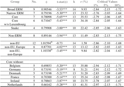
The convergence test is performed on the two groups and reported in Tables 2 and

3. The results for the non-ERM group are our benchmark case. Comparison of the change

in convergence rates between the pre-ERM and ERM periods for both groups has the

following rationale: if the positive interperiod change in the convergence rate for the

ERM group surpasses that of the non-ERM group, then this feature is a supportive

argument for the active role of the ERM in contributing to accelerate inflation

convergence of its member countries.7 When looking at the Core ERM group we found

that the convergence rate increased between the two periods by 13.22%. The same

comparison of the non-ERM group is unfortunately precluded because convergence

coefficient is statistically insignificant in the pre-ERM period. Comparison of

convergence rates alone shows that the Core group is converging during the ERM period

at the rate more than three times larger than the non-ERM group.

These findings allow us to formulate the main result of this paper. There exist

inflation convergence among countries within Europe. It is also evident that the countries

which continuously participated in the narrow ERM bands show a dramatically higher

convergence rate during the ERM period than those staying outside the mechanism.

We now proceed to investigate several additional groups. First, Luxembourg was

currency union with Belgium but exhibits a different rate of inflation. The difference is

insignificant in this analysis because the convergence rate during the ERM period is

compared with that of the previous group, and both rates are found to be essentially

equal. The increase in the convergence rate between the two periods is 11.01%. This

confirms robustness of the main result, and also justifies elimination of Luxembourg from

further analysis.8

We form a narrow ERM group consisting of the founding countries by adding

Italy to the Core ERM group. It is interesting to see that interperiod convergence rate

increased in case of this group by merely 3.69%. Such a result does not come as a

surprise. The Italian lira enjoyed wider fluctuation bands within the ERM and is

historically a currency of higher inflation. Its exclusion from the Core group proved to be

well justified. Alternatively, this could be taken to prove that ERM membership does not

guarantee convergence.

Spain and Portugal were added to the narrow ERM to form the broad ERM

because both are currently members and have tried to lower their national inflation rates

before officially joining the ERM. They did not succeed in this task, and the result is as

we suspected. The broad ERM exhibits the lowest convergence rate at all. This is not

surprising because this group contains very diversified mix of countries with quite

different monetary histories regarding their affiliation with the ERM. Unfortunately the

interperiod change in convergence rate cannot be calculated because of statistical

insignificance of the convergence coefficient during the pre-ERM period.

7 _{This statement should be understood together with the fact that strongest motivation of why the ERM was}

An interesting result is obtained from analysis conducted on a reduced Core

group, referred to as the Snake. The Snake is a group of four countries that formed an

exchange rate arrangement preceding the ERM.9 The creation of the ERM did not bring

these countries an institution of exchange rate peg. The exchange rates of the Snake were

already fixed throughout the pre-ERM period. Thus, the ERM arrangement of fixed

exchange rates should not matter. Interperiod comparison shows that, indeed, the Snake

exhibits an decrease of 6.6% in its convergence rate.

As a control group we use three panels of OECD countries that were not members

of the EU. Panel containing Austria, Sweden, Finland, Switzerland, Norway, Iceland,

United States, Canada, Japan, Australia, New Zealand, and Turkey was analyzed as a

whole as well as divided into European and non-European OECD countries. Convergence

coefficients for the pre-ERM period are insignificant without exception. In the ERM

period the broad panel is insignificant as well. European countries show convergence at

the rate that is comparable with the previously presented group of non-ERM countries.

That means too low in comparison with the ERM countries. Non-European countries

even show divergence of their differentials at the rate of almost 10%. The results support

an active role of the ERM.

In order to test robustness of the analysis, several additional groups were

constructed out of the Core countries in a systematic way. The ERM Core of six countries

was reduced by one country at a time so that six combinations of five Core countries

emerged. Tables 2 and 3 present results of the test for pre-ERM and ERM periods to

8_{Similar comparisons were made also on other pairs of groups differing solely by exclusion of}

answer the question of whether a particular country has some special influence on the

inflation convergence of a certain group.

The convergence coefficients are significant at 5% level for the pre-ERM period

and at the 1% level for the ERM period. When the two periods are compared, all groups

show a similar sharp increase in convergence rates. The only exception is the

convergence rate of the Core without Germany, which exhibits decrease from 45% to

31% over the two periods. Generally, it can be said that eliminating one country out of

the group does not radically affect the group’s convergence path. In other words,

exclusion of a particular country does not affect the robustness of the analysis.

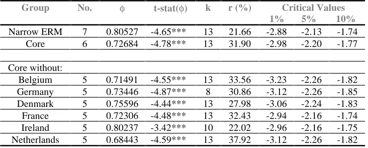
Two more sets of panels were constructed and tested in order to examine whether

inflation convergence within a certain group was affected by specific events. Such events

are the September, 1992, and the August, 1993, crises of the ERM. The original ERM

period was truncated accordingly. The first period begins in 1979:2 and ends in 1992:2.

The second period begins in 1979:2 and ends in 1993:2. The results are presented in

Tables 4 and 5. Convergence coefficients are significant at 1% level in all cases. The

narrow ERM and the Core groups reveal, through the magnitudes of the convergence

rates, that the convergence process was not substantially affected by any of the two major

ERM crises. The systematic part reveals that the convergence rates are not substantially

affected by dropping one country from the Core panel and that the results remain robust.

The Core countries followed very similar convergence paths no matter whether or not the

crisis are excluded.

9

4. Conclusion

This paper examines whether there exists convincing evidence of inflation

convergence within the ERM and whether the ERM helped to accelerate the convergence.

A methodology originally developed to investigate cross-country output convergence was

applied to investigate inflation convergence within the European Union. The analysis is

conducted on logically as well as systematically differentiated groups of countries pooled

together over two basic time periods. These periods cover time span from the late 1950’s

to mid 1990’s with 1979 (inception of the ERM) as a midpoint.

A group of countries that never participated in the ERM serves as a benchmark

case. Results of the test conducted on this group are compared with those of the Core

ERM countries that founded the ERM and never deviated from it. The findings allow us

to formulate the main result of this paper. There exist inflation convergence among

countries within Europe. It is also evident that the countries which continuously

participated in the narrow ERM bands show a dramatically higher convergence rate

during the ERM period than those staying outside the mechanism.

The main result is exposed to a sensitivity analysis. Convergence tests on

modified groups of the ERM countries show robustness of the analysis and justifies the

composition of the Core group. Systematic modification of the Core group itself is

evidence of robustness as well. Eliminating one country from the group does not

seriously affect the magnitude of the convergence rate and the converging path in neither

the pre-ERM nor ERM periods. The influence of the ERM crises is also investigated.

Magnitudes of rates show that the convergence process was not substantially affected by

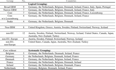
Table 1

Groups of Countries in Each Panel Data Set

Group No. Countries

Logical Grouping:

Broad ERM 9 Germany, the Netherlands, Belgium, Denmark, Ireland, France, Italy, Spain, Portugal Narrow ERM 7 Germany, the Netherlands, Belgium, Denmark, Ireland, France, Italy

Core 7 Germany, the Netherlands, Belgium, Denmark, Ireland, France, Luxembourg Core

w/o Luxembourg

6 Germany, the Netherlands, Belgium, Denmark, Ireland, France

Snake 4 Germany, the Netherlands, Belgium, Denmark

Non-ERM 8 United Kingdom, Greece, Austria, Sweden, Finland, Switzerland, Norway, Iceland

non-EU 12 Austria, Sweden, Finland, Switzerland, Norway, Iceland, United States, Canada, Japan, Australia, New Zealand, Turkey

non-EU, Europe 6 Austria, Sweden, Finland, Switzerland, Norway, Iceland non-EU,

non-Europe

6 United States, Canada, Japan, Australia, New Zealand, Turkey

Core without: Systematic Grouping:

Belgium 5 Germany, the Netherlands, Denmark, Ireland, France Germany 5 the Netherlands, Belgium, Denmark, Ireland, France Denmark 5 Germany, the Netherlands, Belgium, Ireland, France

France 5 Germany, the Netherlands, Belgium, Denmark, Ireland Ireland 5 Germany, the Netherlands, Belgium, Denmark, France Netherlands 5 Germany, Belgium, Denmark, Ireland, France

Table 2

Logical and Systematic Grouping Period 1959:2 - 1979:1

Group No. φ t-stat(φ) k r (%) Critical Values

1% 5% 10%

Broad ERM 9 0.94231 -0.79 13 5.94 -2.75 -2.01 -1.61 Narrow ERM 7 0.82170 -2.57** 10 19.63 -2.69 -1.97 -1.56 Core 7 0.80000 -2.53** 11 22.31 -2.71 -1.98 -1.54 Core

w/o Luxembourg

6 0.79320 -2.43** 11 23.17 -2.70 -1.97 -1.53

Snake 4 0.74812 -2.15** 11 29.02 -2.75 -2.05 -1.64

Non-ERM 8 0.93067 -1.35 11 7.18 -2.78 -2.03 -1.63

non-EU 12 0.96438 -0.82 11 3.63 -2.74 -2.08 -1.69 non-EU, Europe 6 0.95828 -0.78 11 4.26 -2.74 -2.02 -1.62

non-EU, non-Europe

6 0.97190 -0.30 14 2.85 -2.75 -1.98 -1.60

Core without:

Belgium 5 0.76645 -2.61** 10 26.60 -2.67 -1.98 -1.58 Germany 5 0.63781 -3.32*** 10 44.97 -2.69 -1.99 -1.58 Denmark 5 0.85517 -2.04** 7 15.65 -2.74 -1.97 -1.58 France 5 0.78493 -2.44** 10 24.22 -2.69 -1.98 -1.59 Ireland 5 0.74606 -2.42** 11 29.29 -2.72 -2.00 -1.63 Netherlands 5 0.81110 -2.14** 11 20.94 -2.71 -2.01 -1.60 No. means number of countries in a particular group, k denotes number of lags, r denotes a rate of convergence

Table 3

Logical and Systematic Grouping Period 1979:2 - 1994:4

Group No. φ t-stat(φ) k r (%) Critical Values

1% 5% 10%

Broad ERM 9 0.90546 -3.53*** 14 9.93 -2.84 -2.15 -1.72 Narrow ERM 7 0.79196 -5.30*** 13 23.32 -2.76 -2.03 -1.64 Core 7 0.70098 -5.65*** 13 35.53 -2.79 -2.06 -1.65 Core

w/o Luxembourg

6 0.71047 -5.43*** 13 34.18 -2.84 -2.05 -1.64

Snake 4 0.79908 -3.00*** 10 22.42 -2.85 -2.06 -1.63

Non-ERM 8 0.89146 -3.94*** 13 11.49 -2.83 -2.13 -1.75

non-EU 12 1.01594D -0.73 14 1.58 -2.86 -2.10 -1.68 non-EU, Europe 6 0.87701 -4.02*** 13 13.12 -2.82 -2.03 -1.63

non-EU, non-Europe

6 1.10338D -3.45*** 14 9.84 -2.82 -2.04 -1.63

Core without:

Belgium 5 0.69853 -5.20*** 13 35.88 -2.94 -2.12 -1.71 Germany 5 0.73191 -5.19*** 8 31.21 -2.91 -2.12 -1.72 Denmark 5 0.73198 -5.21*** 13 31.20 -2.83 -2.09 -1.69 France 5 0.70300 -5.14*** 13 35.24 -2.82 -2.08 -1.67 Ireland 5 0.78863 -3.87*** 10 23.75 -2.78 -2.07 -1.67 Netherlands 5 0.66162 -5.28*** 13 41.31 -2.97 -2.13 -1.71 No. means number of countries in a particular group, k denotes number of lags, r denotes a rate of convergence

Table 4 Systematic Grouping Period 1979:2 - 1992:2

Group No. φ t-stat(φ) k r (%) Critical Values 1% 5% 10%

Narrow ERM 7 0.79545 -4.66*** 13 22.88 -2.98 -2.17 -1.73 Core 6 0.76665 -4.85*** 8 26.57 -3.02 -2.18 -1.76

Core without:

Belgium 5 0.77640 -4.34*** 8 25.31 -3.00 -2.16 -1.72 Germany 5 0.73439 -4.73*** 8 30.87 -3.33 -2.30 -1.83 Denmark 5 0.73408 -4.66*** 13 30.91 -3.10 -2.20 -1.77 France 5 0.76626 -4.54*** 8 26.62 -3.08 -2.18 -1.69 Ireland 5 0.79625 -3.39*** 10 22.78 -3.09 -2.14 -1.70 Netherlands 5 0.61215 -6.62*** 10 49.08 -3.11 -2.24 -1.75 No. means number of countries in a particular group, k denotes number of lags, r denotes a rate of convergence in %.

***, **, and * denote significance at 1%, 5%, and 10% levels, respectively

Table 5 Systematic Grouping Period 1979:2 - 1993:2

Group No. φ t-stat(φ) k r (%) Critical Values 1% 5% 10%

Narrow ERM 7 0.80527 -4.65*** 13 21.66 -2.88 -2.13 -1.74 Core 6 0.72684 -4.78*** 13 31.90 -2.98 -2.20 -1.77

Core without:

Belgium 5 0.71491 -4.55*** 13 33.56 -3.23 -2.26 -1.82 Germany 5 0.73446 -4.87*** 8 30.86 -3.12 -2.26 -1.85 Denmark 5 0.75596 -4.44*** 13 27.98 -3.06 -2.24 -1.83 France 5 0.72306 -4.48*** 13 32.43 -2.94 -2.16 -1.74 Ireland 5 0.80237 -3.42*** 10 22.02 -2.96 -2.16 -1.75 Netherlands 5 0.68443 -4.59*** 13 37.92 -3.12 -2.26 -1.82 No. means number of countries in a particular group, k denotes number of lags, r denotes a rate of convergence in %.

References

Baxter, M., and Stockman, A., 1989, Business Cycles and the Exchange-Rate Regime: Some International Evidence, Journal of Monetary Economics, 23, 377-400

Bayoumi, T., and Mason, P. R., 1995, Fiscal Flows in the United States and Canada: Lessons for Monetary Union in Europe, European Economic Review, 39, 253-274

Ben-David, Dan, 1995, Measuring Income Convergence: An Alternative Test, Tel Aviv University, Foerder Institute Working Paper 41-95

Ben David, Dan, 1996, Trade Convergence Among Countries, forthcoming: Journal of

International Economics

Barro, R. J., and Sala-i-Martin, X., 1991, Convergence Across States and Regions,

Brookings Papers on Economic Activity, 1, 107-182

Barro, R. J., and Sala-i-Martin, X., 1992, Convergence, Journal of Political Economy, 100, 223-251

Campbell, J. Y., and Perron, P., 1991, Pitfalls and Opportunities: What Macroeconomist Should Know About Unit Roots, NBER Macroeconomics Annual

De Grauwe, P., 1992, Inflation Convergence During the Transition to EMU, Economies

et SociJ_tJ_{s, 26(9-10), 13-32}

De Grauwe, P., 1994, The Economics of Monetary Integration, 2nd ed., Oxford University Press

De Grauwe, P., 1995, The Economics of Convergence Towards Monetary Union in Europe, CEPR Discussion Paper No. 1213

Dickey, D., and Fuller, W. A., 1979, Distribution of the Estimators for Time Series Regressions with a Unit Root, Journal of the American Statistical Association, 74, 427-431

Giavazzi, F., and Giovanninni, A., 1989, Limiting Exchange Rate Flexibility, The MIT Press, Cambridge, Massachusetts

Levin, A., and Lin, Chien-Fu, 1992, Unit Root Tests in Panel Data: Asymptotic and Finite-Sample Properties, University of California - San Diego Discussion Paper 92-23

Papell, D., 1995, Searching for Stationarity: Purchasing Power Parity Under the Current Float, University of Houston Working Paper

Schwarz, G., 1978, Estimating the Dimension of a Model, Annals of Statistics, 6, 461-464