Simulation of Vedic Multiplier in DCT Applications
Vaijyanath Kunchigi
JNTU Hyderabad A.P, INDIA
Linganagouda Kulkarni,
PhD. JNTU Hyderabad
A.P, INDIA
Subhash Kulkarni,
PhD.JNTU Hyderabad A.P, INDIA
ABSTRACT
This paper illustrates the simulation of Vedic multiplier in 2-D 2-DCT. The input data is first divided into NxN blocks, each block s of 8x8 size and 2-D DCT is applied on each of these 8x8 block and 2-D DCT is applied to reconstruct the image. The proposed 2-D DCT design uses Urdhva Tiryagbhyam a Vedic multiplication sutra and the Simulations with MATLAB prove that the proposed design is compared to that of conventional design. Performing DCT computations using Vedic multiplication sutras gives a significant performance even compared to a DCT using conventional. To illustrate our approach, the sample code implements part of JPEG compression routine, performs forward DCT on 8x8 blocks, quantizes coefficients, and performs inverse DCT.
Keywords
Vedic Mathematics; Urdhva Triyakbhyam Sutra; 2-D DCT; Joint Photographic Expert Group (JPEG); Byte
1. INTRODUCTION
The Discrete Cosine Transform (DCT) is a Fourier-like transform, which is widely used in digital signal processing. It was first proposed by Ahmed et al. (1974) [1], and has become the key feature in lossy compression and other DSP-related areas. DCT is known for its high “energy compaction” and decorrelation properties, meaning that the transformed signal can be easily analyzed using few low-frequency components. There are several types of DCT and the most popular is a symmetric presentation and its inverse, these are utilized in JPEG compression routines.
Discrete cosine transform is a powerful tool widely utilized in many applications, especially related to digital signal processing. It has become a de-facto standard in image and video coding algorithms. While the Fourier Transform represents a signal as the mixture of sines and cosines, the Cosine Transform operates only with cosines. The purpose of DCT is to perform “energy compaction” of the input signal and to present the output in the frequency domain. DCT turns out to be a reasonable balance of optimality of input decorrelation and the computational complexity.
The discrete cosine transform (2-D DCT) has become one of the most popular transforms for many image compression applications. The 2-D DCT is computationally intensive and as such there is a great demand for high speed, high throughput and short latency computing architectures. Due to the high computation requirements, the 2-D DCT processor design has been concentrated on small non-overlapping blocks (typical 8x8 or 16x16). To meet the real-time audio, image and video-processing requirement, DCT and inverse DCT (IDCT) are needed [5]. There are various algorithms for computation of Discrete Transforms that have been developed over the years [2-6].
This paper is organized as follows. Section II gives an overview of 2-D DCT. Following section III gives the overview of Vedic Mathematics. Section IV explains the
Vedic Multiplier & Transform algorithms. Section V presents the simulation of 2-D DCT and its simulated result is shown. Conclusion is given in section VI.
2. DISCRETE COSINE TRANSFORM
The discrete cosine transform is a fast transform. It is a widely used and robust method for image Compression. It has excellent compaction for highly correlated data. DCT has fixed basis images DCT gives good compromise between information packing ability and computational complexity. It transforms the input data into a format to reduce interpixel redundancies in the input image. Transform coding techniques use a reversible, linear mathematical transform to map the pixel values onto a set of coefficients, which are then quantized and encoded. The key factor behind the success of transform-based coding schemes is that many of the resulting coefficients for most natural images have small magnitudes and can be quantized without causing significant distortion in the decoded image. DCT separates images into parts of different frequencies where less important frequencies are discarded through quantization and important frequencies are used to retrieve the image during decompression. Compared to other input dependent transforms, DCT has many advantages: (1) It has been implemented in single integrated circuit; (2) It has the ability to pack most information in fewest coefficients; (3) It minimizes the block like appearance called blocking artifact that results when boundaries between sub-images become visible.
The Discrete Cosine Transform (DCT) is one of many transforms that takes its input and transforms it into a linear combination of weighted basis functions. A 2-D DCT is defined as
..(1)
There is also an Inverse DCT which just takes the DCT coefficients and multiplies them with the basis functions and adds all of them together. Surprisingly, the IDCT is very similar to the DCT. And inverse transform is defined as
.. (2) These functions are called the basis functions of the DCT. The DCT coefficients, then, can be regarded as the weights applied to each basis function. For 8-by-8 matrices, the 64 basis functions called masks are obtained. The cosine values is computed using the 64 masks
3. VEDIC MATHEMATICS
structured, both within themselves and in relation to each other. Some documents, called ‘Ganita sutras’ (the name ‘ganita’ means mathematics), were devoted to mathematical knowledge. Sri Bharati Krishna Tirtha Maharaj, who is generally considered the doyen of this discipline, in his seminal book Vedic Mathematics, wrote about this special use of sutras[7]. Vedic Mathematics" was the name given by him. He was the person who collected lost formulae from the writings of "Atharwa Vedas" and wrote them in the form of Sixteen Sutras and thirteen sub-sutras. Vedic Mathematics is based on 16 sutras dealing with mathematics related to arithmetic, algebra, and geometry.
4. VEDIC MULTIPLIER & TRASSFORM
ALGORITHM
Multiplication is a fundamental operation in most signal processing algorithms. Multipliers have large area, long latency and consume considerable power. Fast multipliers are essential parts of digital signal processing systems. The speed of multiply operation is of great importance in digital signal processing as well as in the general purpose processors today, especially since the media processing took off.
4.1 Vedic Multiplication
In this section, we explore three Vedic multiplication sutras. Out of two there is one generic method which can be applied to all cases whereas other two are for special cases which are simpler to deal with. As the main purpose of Vedic Mathematics is to be able to solve complex calculations by simple techniques. The formulas being very short their practical application becomes very simple.
4.1.1 Nikhilam Sutra
The sutra basically means start from the left most digit and begin subtracting ‘9’ from each of the digits; but subtract ‘10’ from the last digit. The meaning of the sutra is “all from 9, last from 10. here “last” indicates digit at unit place which is to be subtracted from 10 and “all” indicates digit at subsequent higher places which are to be subtracted from 9.” This sutra is special used for base multiplication i.e, near the base. Base means 10, 100, 1000 etc.
4.1.2 Urdhva-tiryagbhyam
As seen in previous section the Nikhilam sutra is for special cases, whereas Urdhva-tiryagbhyam [8], is the general formula which is applicable to all cases of multiplication. Urdhva Triyagbhyam means “Vertically and Crosswise”, which is the method of multiplication followed in this paper. Digital multipliers are indispensable in the hardware implementation of many important functions such as DFT, DWT, FFT etc [9-11]. The DCT (Discrete Cosine transform) performs spatial compression and decompression of data and these functions are performed using Vedic algorithms. The proposed Vedic multiplier significantly improves the computational speed involved in multiplication operations of the image processing. The other advantage of Vedic algorithm it can be easily realized on hardware. In multipliers based on the Vedic algorithm, there is no visible difference between image reconstructed using Vedic multipliers and image reconstructed using standard multipliers.
5. 2-D DCT SIMULATION RESULTS
AND DISCUSSION
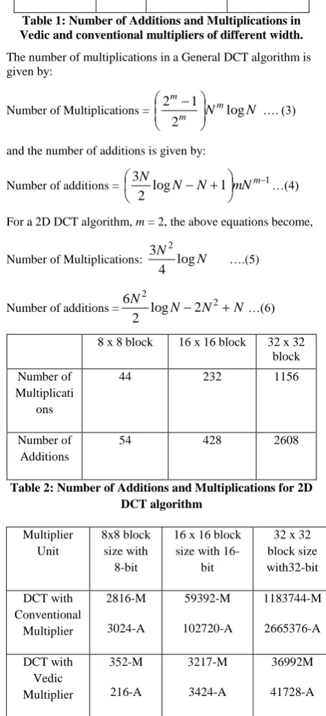
The number of additions and multiplications in a Vedic multiplier versus the ALU multiplier is given in Table 1.
Multiplier Unit
8-bit 16-bit 32-bit
Conventional 64-M
56-A
256-M
240-A
1024-M 1022-A
Vedic 8-M
4-A
16-M
8-A
32-M
[image:2.595.321.537.71.208.2]16-A
Table 1: Number of Additions and Multiplications in Vedic and conventional multipliers of different width.
The number of multiplications in a General DCT algorithm is given by:
Number of Multiplications = m
N
mN
m
log
2
1
2
…. (3)and the number of additions is given by:
Number of additions =
log
1
12
3
mmN
N
N
N
…(4)
For a 2D DCT algorithm, m = 2, the above equations become,
Number of Multiplications:
N
log
N
4
3
2….(5)
Number of additions =
N
N
N
2
N
2
2
log
2
6
…(6)8 x 8 block 16 x 16 block 32 x 32 block Number of
Multiplicati ons
44 232 1156
Number of Additions
[image:2.595.311.548.186.706.2]54 428 2608
Table 2: Number of Additions and Multiplications for 2D DCTalgorithm Multiplier Unit 8x8 block size with 8-bit
16 x 16 block size with
16-bit
32 x 32 block size with32-bit DCT with Conventional Multiplier 2816-M 3024-A 59392-M 102720-A 1183744-M 2665376-A DCT with Vedic Multiplier 352-M 216-A 3217-M 3424-A 36992M 41728-A
Table 3: Number of Additions and Multiplications for 2D DCT algorithm with conventional versus vedic multiplier
size can be used in combination with the 16 bit of 32 bit multiplier depending upon the number of digits used for the stored in the multiplier.
Transform coding algorithms usually start by partitioning the original image into sub images (blocks) of small size (usually 8 × 8). For each block the transform coefficients are calculated, effectively converting the original 8 × 8 array of pixel values into an array of coefficients within which the coefficients closer to the top-left corner usually contain most of the information needed to quantize and encode (and eventually perform the reverse process at the decoder’s side) the image with little perceptual distortion. In the JPEG image compression algorithm, the input image is divided into 8-by-8 or 16-by-16 blocks, and the two-dimensional DCT is computed for each block. The DCT coefficients are then quantized, coded, and transmitted. The JPEG receiver (or JPEG file reader) decodes the quantized DCT coefficients, computes the inverse two-dimensional DCT of each block, and then puts the blocks back together into a single image. For typical images, many of the DCT coefficients have values close to zero; these coefficients can be discarded without seriously affecting the quality of the reconstructed image. JPEG Process: Original image is divided into blocks of 8 x 8. Pixel values of a black and white image range from 0-255 but DCT is designed to work on pixel values ranging from -128 to 127 . Therefore each block is modified to work in the range. Equation(1) is used to calculate DCT matrix. DCT is applied to each block by multiplying the modified block with DCT matrix on the left and transpose of DCT matrix on its right. Each block is then compressed through quantization. Quantized matrix is then entropy encoded. Compressed image is reconstructed through reverse process. Inverse DCT is used for decompression.
[image:3.595.321.534.76.375.2]The design flow starts with the MATLAB environment for the computation of image pixels. The image is segmented into 8x8. The time domain coefficients are converted into spectral coefficient. Similarly the computation of 2-D DCT is performed and its functional verification is carried out. The output of 8x8 block produces 64 DCT coefficients which is stored in a matrix. The IDCT is performed to recreate the input image.
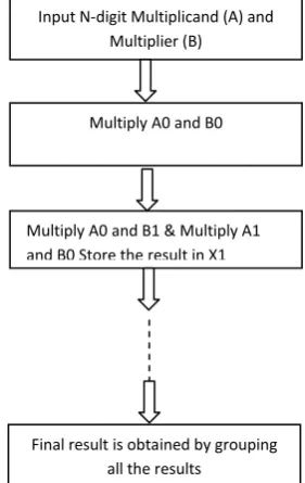
[image:3.595.98.239.509.732.2]Fig 1: Vedic Multiplier Flow chart
Fig 2: Design Flow of the 2-D DCT & its Inverse DCT
The flow chart in fig 2 shows, the computation of two-dimensional DCT of 8-by-8 blocks in the input image. WE obtain 64 DCT coefficients in each block, and then reconstruct the image using the two-dimensional inverse DCT of each block.
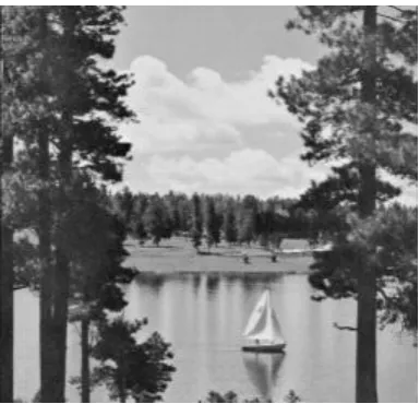
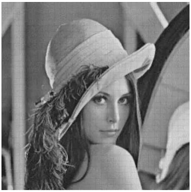
The input images are shown in Figs. 3a and 4a. The Vedic multiplier is implemented along with the 2D DCT. The purpose of using MATLAB for implementing the Vedic multiplier is only for simulation of the hardware. In practical applications, the Vedic multiplier must be implemented in hardware along with DCT for better efficiency. Otherwise, implementation-using MATLB will turn very costly. In this work, usage of vedic multiplier is simulated for studying the output of images from the DCT algorithm.
As depicted in Fig. 2, first reading the input image and splitting the image matrix into the smaller matrices of size 8x8 implement the 2D DCT. The 8x8 matrix is transformed using DCT. The multiplications used in the DCT algorithm are carried out using the Vedic multiplier instead of traditional ALU multiplier of a computer processor except for the single digit multiplication.
One of the challenges one has to face while carrying out the multiplications inside the DCT is handling of the multiplication of real numbers, especially the number that are between 0 and 1. It is a challenge because; the Vedic multipliers are generally available for multiplying integer numbers. In this work, the real numbers between 0 and 1 are encountered when using the alpha coefficients and cosine values of the DCT formulation.
In this work, three types of Vedic multipliers are simulated, namely, single digit, two digit and three digit multipliers. The single digit multiplier is nothing but the traditional ALU multiplier, where as the other two are implemented using procedure laid as per Vedic mathematics. The alpha and cosine values are multiplied by three different numbers, vis Input N-digit Multiplicand (A) and
Multiplier (B)
Multiply A0 and B0
Store the result in X0
Multiply A0 and B1 & Multiply A1 and B0 Store the result in X1
Final result is obtained by grouping all the results
Read the Input Image
Input Image is divided into 8x8 blocks
Computation of DCT on each 8x8 block
Create complete matrix using all the calculated values of 8x8 blocks
Create the image using the obtained matrix Calculate the size of the input
image
Computation of IDCT on each 8x8 block
10,100 and 1000 and rounded off to nearest integer in order to tryout the result for different accuracies in this work. The magnified alpha and cosine values are de-magnified at appropriate places inside the DCT and inverse DCT. When the alpha and cosine valuesare multiplied by the 10,100 and 1000 and rounded off to nearest integer, reduction in computational complexity can be estimated from table 3, depending up on the number of digits of the number and the block size used for DCT.
After carrying out the DCT, the matrices are transformed back to original matrices using inverse DCT. Here again, the alpha and cosine values are multiplied by three different numbers, vis 10, 100 and 1000 and rounded off to nearest integer. The output images of this process are shown below as Figs. 3b, 3c and 3d; and Figs 4a, 4b and 4c.
One can notice the difference in the quality of the images visually. By multiplying the alpha and cosine values by 10, only one digit after the decimal point is extracted and the number becomes single digit after rounding off. It becomes and two and three digits if multiplied with 100 and 1000. The Vedic multiplier to be used for two and three digit number is different and hence requires different computational resources. Hence lower the number of digits, the better it is. However, the gain in the savings from hardware resources is at the cost of the output images. Hence one should use trade-off in deciding the number of digits in multiplication and the output image quality.
The single digit multiplier yields the poor quality image where as the one with three digits yields highest quality among the three cases used.
[image:4.595.334.526.71.263.2]One can notice the grid for the single and two digit multipliers. The grid can be observed as dark lines in the case of single digit multiplier and it is light in case of two digit multiplier. This is due to the reason that, the pixel values gradually reduces towards zero as the frequencies increase towards the end of the block horizontally and vertically, when an inverse DCT is taken. The reason behind this type of behavior is the loss of data when the alpha and cosine values are approximated with just one digit while truncating the other digits. This phenomenon becomes prominent when the frequencies increase. This effect becomes less significant when two digits and more make the approximation.
[image:4.595.333.526.307.502.2]Fig. 3a: Input Image 1 to DCT
[image:4.595.70.264.517.713.2]Fig. 3b: Output Image from DCT using Single Digit Multiplier
Fig. 3c: Output Image from DCT using Two Digit Multiplier
[image:4.595.333.526.545.730.2]Fig. 4a: Input Image 1 to DCT
[image:5.595.70.264.75.284.2]Fig. 4b: Output Image from DCT using Single Digit Multiplier
Fig. 4c: Output Image from DCT using Two Digit Multiplier
Fig. 4d: Output Image from DCT using Three Digit Multiplier
6. CONCLUSION
This paper presented the simulation of 2-D DCT and 2-D IDCT using Vedic multiplication sutra. The first input image is divided into blocks, each block is of size 8x8 and 2-D DCT is applied on each of these 8x8 blocks and 2-D IDCT is applied to reconstruct the image. The proposed 2-D DCT using Vedic multiplication sutra called “Urdhva Tiryagbhyam” and simulation with MATLAB shows the proposed simulation shows significant performance compared to the conventional DCT. To illustrate approach presented in this work, three cases are considered, namely first case is using single digit Vedic Multiplier, second case is using two digits Vedic Multiplier and third case is using three digits Vedic multiplier. It is shown that the three digit Vedic Multiplier yields the best results among the three cases, but is computationally costly. In future, the blocks size will be varied to 16x16 and 32x32 to study the effects of the image quality and the factors associated with the image quality will be computed for better comparison.
7. REFERENCES
[1] N. Ahmed, T. Natarajan, and K. R. Rao, “Discrete cosine transforms, IEEE Trans. Comput., vol. 23, pp. 90–93, Jan. 1974.”
[2] Thuyen Le and Manfred Glesner,” Flexible Architectures for DCT of Variable-Length Targeting Shape-Adaptive Transform”, IEEE Transactions on Circuits and Systems For Video Technology, VOL. 10, NO. 8, December 2000.
[3] Liu Yuejun, Su Jing and Liu Feng ,” Research on Information Hiding System based on DCT Domain”, 2010 Second International Conference on Computer Modeling and Simulation, 978-0-7695-3941-6/10 IEEE, DOI10.1109/ICCMS.2010.342, 2010.
[4] Jie Liang and Trac D.Tran,” Fast Multiplierless Approximation of the DCT with the Lifting Scheme”, IEEE Transaction on Signal Processing, Submitted; FEB. 2001.
[image:5.595.70.265.201.477.2] [image:5.595.70.265.519.715.2]Video Codecs”, Arlington, Virginia, Int. ASIC/SOC Conference,pp. 203-207, September 2001.
[6] Clay Gloster, Jr., Wanda Gay, Michaela Amoo, and Mohamed Chouikha,” Optimizing the Design of a Configurable Digital Signal Processor for Accelerated Execution of the 2-D Discrete Cosine Transform”, Proceedings of the 39th Hawaii International Conference on System Sciences – 2006.
[7] Jagadguru Swami Sri Bharath, Krsna Tirathji, “Vedic Mathematics or Sixteen Simple Sutras From The Vedas”, Motilal Banarsidas, Varanasi (India), 1986.
[8] “A Reduced-Bit Multiplication Algorithm For Digital Arithmetic” Harpreet Singh Dhilon And Abhijit Mitra, International Journal of Computational and Mathematical Sciences, Waset, Spring, 2008.
[9] Anvesh kumar,Ashish Raman,R K Sarin,Arun Khosla “Small Area Reconfigurable FFT Design by Vedic Mathematics ” in Proc IEEE ICAAE’10,Singapoure, vol 5,pp. 836-838,Feb. 2010
[10] Shripad Kulkarni, “Discrete Fourier Transform (DFT) by using Vedic Mathematics”Papers on implementation of DSP algorithms/VLSI structures using Vedic Mathematics, 2006, www.edaindia.com, IC Design portal.
[11] “Lifting Scheme Discrete Wavelet Transform Using Vertical and Crosswise Multipliers” Anthony O’Brien and Richard Conway, ISSC, 2008, Galway, June 18-19. [12] S.G. Dani, Vedic Maths’: facts and myths, One India One