A New Method to Grid Noisy cDNA Microarray Images Utilizing Denoising Techniques

A New Method to Grid Noisy cDNA Microarray Images

Utilizing Denoising Techniques

Islam A. Fouad

Biomedical Technology Dept. SALMAN BIN A.Aziz University

K.S.A., Al-Kharj

Mai S.Mabrouk

Biomedical Engineering Dept. MUST University Egypt, 6th of October

Amr A. Sharawy

Biomedical Engineering Dept. Cairo University

Egypt, Cairo

ABSTRACT

DNA Microarray is an innovative tool for gene studies in biomedical research, and its applications can vary from cancer diagnosis to human identification. It is capable of testing and extracting the expression of large number of genes in parallel. The gene expression process is divided into three basic steps: gridding, segmentation, and quantification. Automatic gridding; which is to assign coordinates to every element of the spot array, is considered the most challenging phase of microarrays image processing.

For processing of microarray images, a new, automatic, fast and accurate approach is proposed for gridding noisy cDNA microarray images. In the real world, microarray image doesn’t reflect measures of the fluorescence intensities for the dye of interest only, as different kinds of noise and artifacts can be observed. In this paper, a novel gridding method based on projection is developed accompanied by a pre-processing, post-processing, and refinement steps for noisy microarray images. Results revealed that the proposed method is used with high accuracy and minimal processing time and can be applied to various types of noisy microarray images.

Keywords

noisy microarray image, gridding, projection, pre-processing, post-processing, refinement.

1.

INTRODUCTION

DNA Microarray is an innovative tool for gene studies in biomedical research. It is capable of testing and extracting the expression of large number of genes in parallel. Microarray applications can vary from cancer diagnosis to human identification.

Thousands of individual genes can be spotted on a single square inch slide. Each gene is single stranded, amplified in number, and put on the slide to form a spot. Sample solution has to be prepared as well. Messenger RNA, the working copies of genes within cells and thus an indicator of which genes are being used in these cells, is purified from cells of a particular type. The RNA molecules are then labeled by attaching a fluorescent dye that allows us to detect them later, and added to the DNA dots on the microarray.

Due to a phenomenon termed base-pairing, RNA will stick to the gene it came from. This process is called hybridization. After washing away all of the unstuck RNA, light is shone over the microarray and it is scanned by optical detector devices to get a fluorescent image.

Processing of a DNA microarray image is a critical step in a microarray experiment [1].There are three basic steps in the processing of a microarray image [2]. The first step, gridding,

is to assign coordinates to every element of the spot array. The second step, segmentation, is to classify a group of pixels as spot pixels. The third step, quantification, deals with measuring the intensity of the spot signal and the background. Gridding is the primary task of DNA microarray image analysis; therefore it is a prerequisite for follow-up to microarray analysis.

Major work has been presented in the domain of microarray image gridding. Li Yi-bo [3] uses a predefined image filter to grid the sub-array image. Hirata J R [4] introduces a technique using morphological operators to perform automatic gridding procedures for sub-grids and spots. G. Antoniol [5] applies markov random field approach that requires user input the size of the spot, and the number of rows and columns. J.Buhler [6] describes a semi-automatic system which mainly focuses on the problem of finding individual spot with high accuracy. A.Jain [7] describes a system for microarray gridding and quantitative analysis that imposes different kinds of restrictions on the print layout. This method requires the rows and columns of all grids to be strictly aligned.

A perfect microarray image should only reflect measures of the fluorescence intensities for the dye of interest [8] and should have the following properties:

• All the sub-grids have the same size and the spacing between them is regular.

• The location of the spots is centered on the intersections of the lines of the sub-grid. • The shape and size of the spots are perfectly

circular and the same for all the spots.

• The location of the grid is fixed in images for a given type of slides.

• No dust or contamination is on the slide. • There is minimal and uniform background

intensity across the image.

However, in the real world, almost no real microarray image meets all the above criteria. In fact, there are frequently observed variations on the spot position, irregularities on the spot size and shape. Different kinds of noise and artifacts [9] can be seen in the microarray images. Black regions around the image mean that some of the spots have been lost during the scanning. Dust particles all around the image, which are seen as bright, irregular points around the image. There are regions with a high level of background illumination. This makes image processing more challenging. Those are some of the factors that the image processor unit should consider during the process of extracting spot intensities of a microarray image.

paper. Experiment shows that this method can deal with various kinds of noisy microarray images, with high accuracy. The paper is organized as follows: a brief introduction is presented in this section, section 2 presents the used materials, section 3 summarizes the proposed gridding method for various cDNA microarray noisy images and section 4 discusses the results of the applied algorithm on microarray data set images. Conclusions and future work are presented in section 5.

2.

MATERIALS

To test the proposed method, fifty images have been selected from different sources, and have different scanning resolutions, and different noise types, in order to study the flexibility of the proposed method to detect spots with different sizes and features.

The first group consists of a set of images drawn from Stanford Microarray Database (SMD), and corresponds to a study of the global transcriptional factors for hormone treatment of Arabidopsis thaliana samples [10].

The second group consists of a set of images from Gene Expression Omnibus (GEO) and corresponds to the Atlantic salmon head kidney study [11].

Depending on the degree of noise, four types of DNA microarray images are analyzed. In this work, Matlab is used for data analysis and technical computing as it is a high performance and powerful tool. The P.C used has a processor: Intel(R) Core (TM) i5 – 2.27 G Hz. and the used Matlab version is (R2012b) and its Image Processing Toolbox which supports an extensive range of image processing operations [12].

A novel gridding method using projection technique is proposed. This method is useful to eliminate various types of noise occurred in microarray images.

3.

METHODS

3.1

Pre-processing the Noisy Image

3.1.1

Global Background Noise Correction

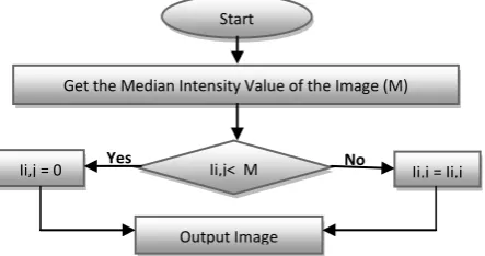
The first step is to remove noise which has gray values on the black background. This can be achieved by getting the median intensity value of the image, and then check each pixel value in the image, and compare this value with the obtained median value. If the pixel intensity value is less than the median value, it will be set to zero. Otherwise, the pixel value is remained as it is. This is shown in Figure 1.

Fig 1: Flowchart of Global Background Noise Correction.

Where, Ii,jis the intensit alue of the i el in the i ro and the column.

3.1.2

Contrast Enhancement

Because of the low-intensity features that are not well distinguishable from the background in most of the microarray images, it's important to develop a new method to improve the contrast between the foreground (spots) and the background. That's can be achieved by applying histogram equalization [12, 13, 14]. Unfortunately, an additive noise (small white spots) appeared on the background which can be eliminated using wiener filter [12, 13,14].

3.1.3

Remove the Large Flare Noise

First erosion [12, 15] operator with a structuring element (In experiment se = 7) is applied to remove foreground spots. Then apply image reconstruction [12, 13] to the result background. An image with less noise is obtained by subtracting resulted background from original image. This is mainly to remove large flare noise. After that, morphological opening with a structuring element (In experiment se = 4) is applied to remove small spikes in the image. Apply image reconstruct again to the result image. This is shown in Figure 2.

Fig 2: Flowchart of Flare Noise Removal.

3.2

Projection Profile Method

To perform this method, a binary image is obtained by applying canny edge detection technique [16, 17]. Then, the detected spots are filled through performing region filling operation. Despite canny detector is one of the best detectors that suppresses noise, it couldn't detect some spots well in the image, as it produces some incomplete regions which is difficult to be filled. To overcome this problem; morphological opening (erosion then dilation) is applied to the resulted binary image [15]. In order to obtain the horizontal intensity projection profile H P(y) of the image [18] f(x,y), the sum of intensity values are calculated at each pixel along the x-axis for each row, which is defined as follow:

H P(y) =

Where, image size is X × Y, HP(y) represents the horizontal projection signal.

Start

Get the Median Intensity Value of the Image (M)

Yes _{Ii,j< M} No

Ii,j = Ii,j Ii,j = 0

Output Image

Apply Morphological Erosion (se = 7)

Reconstruct Image

Subtract Reconstructed Image from the Input Image to Remove the Flare Noise

Apply Morphological Opening to Remove Small Spikes

Reconstruct Image

The negative peaks of the profile are detected that correspond to the positions of the vertical grid lines. The actual image contains noise and other factors, so if directly use the above method for gridding, it may cause the phenomenon of missing or redundant grid lines. Therefore, to grid the image correctly, de-noising and refinement of the projection profile is required. Finally, to determine the horizontal grid lines, the image matrix is transposed for only one time, and then all the previous steps are repeated starting from obtaining the projection profile.

3.3

Post-processing Technique

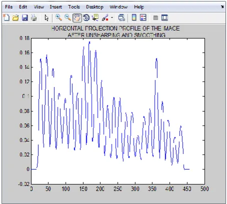
As presented before, it was found that there're a lot of sharp spikes may be appeared on the image profiles, which was understood that they're false peaks. So, before performing the computations, a new approach is proposed to enhance and de-noise the calculated profile by applying two filters: un-sharpening and smoothing. The smoothing filter size value was set to 7 according to experiment.

3.4

Gridding Refinement

The proposed method has high accuracy, but in practice, no methods can grid entirely correct. Therefore, we proposed a grid correction method as in the following steps:

• Apply autocorrelation to the mean horizontal profile [12, 18], where, autocorrelation [19] is the cross-correlation of a signal with itself. • Get the maximum peak indicies from the

autocorrelated profile.

• Calculate an estimated period, which is a distance between two adjacent spot centers. • By experiment, Compare between the obtained

estimated period (E) and the distance between each two adjacent minimum peaks (M) obtained.

• When M < 0.5 E, there will be a mistakenly drawn line. Therefore, take a new index (inew) between the two adjacent minimum peak indices (i, i+1), where,

inew = (i + (i+1)) /2.

• Eliminate the fault indices (i,i+1), and then, inew = i.

4.

RESULTS AND DISCUSSIONS

The proposed gridding method was implemented on a number of noisy microarray images from two different sources; Stanford Microarray Database (SMD) and Gene Expression Omnibus (GEO).

The cropped microarray image is composed of the same number of rows and columns of spots. Depending on the degree of noise and how the spots are expressed, four kinds of images are used:

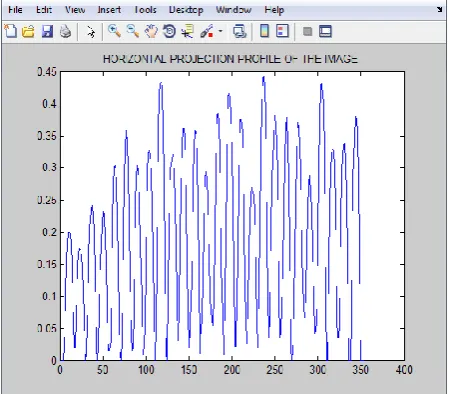
High quality images (very good image).

 Figure 3 shows the very good image.

 Figure 4 shows the very good image after background noise correction.

 Figure 5 shows the very good image after contrast enhancement.

 Figure 6 shows the very good image after removing flare noise.

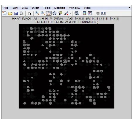
 Figure 7 shows the horizontal projection profile of the very good image.

 Figure 8 shows the profile of the very good image after un-sharpening and smoothing.

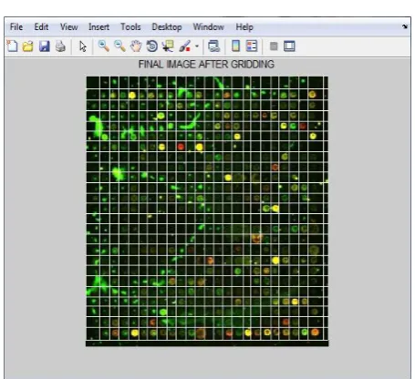
 Figure 9 shows the gridded very good image. Moderate quality images (good image).

 Figure 10 shows the good image.

 Figure 11 shows the good image after background noise correction.

 Figure 12 shows the good image after contrast enhancement.

 Figure 13 shows the good image after removing flare noise.

 Figure 14 shows the horizontal projection profile of the good image.

 Figure 15 shows the profile of the good image after un-sharpening and smoothing.

 Figure 16 shows the gridded good image. General quality images (fair image).

 Figure 17 shows the fair image.

 Figure 18 shows the fair image after background noise correction.

 Figure 19 shows the fair image after contrast enhancement.

 Figure 20 shows the fair image after removing flare noise.

 Figure 21 shows the horizontal projection profile of the fair image.

 Figure 22 shows the profile of the fair image after un-sharpening and smoothing.

 Figure 23 shows the gridded fair image. Bad quality images (poor image).

 Figure 24 shows the poor image.

 Figure 25 shows the poor image after background noise correction.

 Figure 26 shows the poor image after contrast enhancement.

 Figure 27 shows the poor image after removing flare noise.

 Figure 28 shows the horizontal projection profile of the poor image.

 Figure 29 shows the profile of the poor image after un-sharpening and smoothing.

 Figure 30 shows the gridded poor image.

Fig 4: Very Good Image after Background Noise Correction.

Fig 5: Very Good Image after Contrast Enhancement.

Fig 6: Very Good Image after Removing Flare Noise.

Fig 7: Horizontal Projection Profile of the Very Good Image.

Fig 8: Profile of the Very Good Image after Un-Sharpening and smoothing.

Fig 10: Good Image.

Fig 11: Good Image after Background Noise Correction.

Fig 12: Good Image after Contrast Enhancement.

Fig 13: Good Image after Removing Flare Noise.

Fig 14: Horizontal Projection Profile of the Good Image.

Fig 16: Gridded Good.

Fig 17: Fair Image.

Fig 18: Fair Image after Background Noise Correction.

Fig 19: Fair Image after Contrast Enhancement.

Fig 20: Fair Image after Removing Flare Noise.

Fig 22: Profile of the Fair Image after Un-Sharpening and Smoothing.

Fig 23: Gridded Fair Image.

Fig 24: Poor Image.

Fig 25: Poor Image after Background Noise Correction.

Fig 26: Poor Image after Contrast Enhancement.

Fig 28: Horizontal Projection Profile of the Poor Image.

Fig 29: Profile of the Poor Image after Un-Sharpening and Smoothing.

Fig 30: Gridded Poor Image.

The accuracy (A) of the applied gridding method on a specified input image, having NTotal Spots, can be calculated as follows:

A = (NCorrect Spots / NTotal Spots) *100 %. (2) Where, NCorrect Spots, NTotal Spots indicates the number of spots

correctly gridded and the total number of spots in the image respectively.

Table 1.Comparison ofthe ProposedMethod with Other MethodsAccuracy.

TYPE OF IMAGE

Accuracy %

Proposed Method

BassimAlha didi et al

Deepa J et al (SE = 4, optimum sub-image = 100)

Very Good

100% 100% 35%

Good 98.6% 98% 55%

Fair 99.13% 30% 69%

Poor 97.9% 60% 50% According to results obtained in this work, it is found that the proposed method provides the highest accuracyas shown in Table 1. Also, it is observed that there is no method practically can grid entirely in a correct way. Therefore, pre-processing, post-pre-processing, and refinement steps as used in this work, effectively can enhance the contrast and eliminate various kinds of noise in the image. This applicable method can correctly grid all the four types of microarray images without any human intervention.

By comparing our method with other methods as those implemented by Deepa J and Tessamma Thomas [20] and BassimAlhadidiet al [21], it was found that our method is more accurate and can grid various types of noisy images correctly as it mainly deals with noisy images. The other two methods have accuracy ranges differ according to the type of noise and the spots size in each image. Deepa J et al method seems to be a semiautomatic gridding method as the accuracy of the results differs according to the values of the selected optimum sub-imageand the structure element (SE) of the opening applied in their algorithm.

It should be noted that the processing time for the gridding of the four various types of microarray images, was lower than 6 sec. (processor: Intel(R) Core (TM) i5 – 2.27 G Hz), rendering the technique a valuable tool for a fully automated microarray image processing application.

5.

CONCLUSION

post-processing, and refining the microarray image before performing the gridding step. The processing time is minimal providing that the developed method is considered as an effective tool for the demanding task of microarray image processing. The next phase of this work is to extract the spot from the background, enhance the microarray image and calculate the intensity for each spot.

6.

REFERENCES

[1] Hunter P...2003. Microarray data analysis: Separating the curd from the whey. Scientist, 50-1.

[2] Jouenne V. Y...2001. Critical Issues in the Processing of cDNA Microarray Images. Virginia Polytechnic Institue. [3] Li Yi-bo..2004. Study of gridding gene chip images

based on Genetic algorithm and deformable template. Tianjin: Hebei University of Technology.

[4] Hirata J. R., Barrera J., Hashimoto R. F..2001. Microarray Gridding by Mathematical Morphology. [C]//Proceeding of XIV, Brazilian Symposium on Computer Graphics and Image Processing.

[5] G. Antoniol and M. Ceccarelli.2004. A Markov Random Field Approach to Microarray Image Gridding. Proc. 17th Int’l Conf.Pattern Recognition, 550-553.

[6] J.Buhler, T.Ideker and D.Haynor. Dapple.2000. Improved Techniques for Findings Spots on DNA Microarrays. Technical ReportUWTR 2000-08-05, University of Washington.

[7] A.Jain, T.Tokuyasu, A.Snijderts, R.Segraves, D.Albertson and D.Pinkel.2003. Fully Automatic Quantification of Microarray Image Data. Genome Res., 12(2), pp.325 – 332.

[8] Stefano Lonardi, Yu Luo.2004. Gridding and Compression of Microarray Images. Computational Systems Bioinformatics Conference, CSB 2004. Proceedings, IEEE, 16-19, pp.122-130.

[9] T. Tu..2002. Quantitative noise analysis for gene expression microarray experiments. Proc. Natl. Acad. Sci., 99, 14031-6.

[10]Stanford Microarray Database (SMD;

http://smd.stanford.edu/)

[11]Rise ML, Jones SR, Brown GD, von Schalburg KR.2004. Microarray analyses identify molecular biomarkers of Atlantic salmon macrophage and hematopoietic kidney response to Piscirickettsiasalmonis infection. Physiol Genomics 15;20(1):21-35.PMID:15454580

(http://www.ncbi.nlm.nih.gov/geo/query/acc.cgi?acc=GS E1031)

[12]Matlab (R2012b) Image Processing Toolbox, Signal Processing Toolbox.

[13]Rafael C. Gonzalez and Richard E.Woods. Digital Image processing, Second Edition.

[14]AcharyaTinku, Ray AjoyK.. 2005. Image Processing Principles and Applications. John Wiley & Sons, Inc.. [15]Y. Wang, F. Y. Shih, and M. Ma.2005. Precise gridding

of microarray images by detecting and correcting rotations in sub-arrays. In proceedings of Sixth Inter. Conf. on Computer Vision, Pattern Recognition and Image Processing, Salt Lake City, UT.

[16]J.F. Canny.1986. A computational approach to edge detection. IEEE Trans Pattern Analysis and Machine Intelligence, 8(6), pp.679-698.

[17]Li Qin, Luis Rueda, Adnan Ali and AliouneNgon.2005. Spot Detection and Image Segmentation in DNA Microarray Data. Appl. Bioinformatics, 4(1), pp. 1-11. [18]J.Angulo and J.Serra.2003. Automatic analysis of DNA

microarray images using mathematical morphology. Bioinformatics, 19(5), pp.553-562.

[19]Patrick F. Dunn.2005.Measurement and Data Analysis for Engineering and Science, New York: McGraw–Hill, ISBN 0-07-282538-3

[20]DeepaJ, and Tessamma Thomas.2009. “Automatic Gridding of DNA Microarray Images using Optimum Subimage”, International Journal of Recent Trends in Engineering, Vol. 1, No. 4.