Image Segmentation using Weighted Average Local Histogram

(1)

Image Segmentation using Weighted Average

Local Histogram

Imran Hassan

Assistant Engineer

Bangladesh Power Development Board

Abrar Hussain

Lecturer

Southern University Bangladesh

ABSTRACT

The prime objective of this paper is to implement an efficient improved color image segmentation method using local histogram and region merging technique. The goal of image segmentation is to cluster pixels into salient image regions, i.e. regions corresponding to individual surfaces, objects or natural parts of objects. Segmentation can be used for object recognition, occlusion boundary estimation within motion or stereo systems, image compression, image editing or image database look-up. Usually image segmentation is an initial and vital step in a series of processes aimed at overall image understanding. There are various techniques for image segmentation. In this research paper, a thorough work has done on the average local histogram of three different color spaces RGB, HSV & Lab. After that k-means clustering and labeling have done on the image for final segmentation.

General Terms

Image Segmentation, Weighted Average Local Histogram.

Keywords

Local Histogram, K-means Clustering, Fuzzy Min-Max Clustering.

1 INTRODUCTION

Image is an important object in any interface related with computer. To understand an image, one needs to isolate the objects in it and find relation among them. Then there is a need of image segmentation. Image segmentation [1, 2] is an essential process for most subsequent image analysis tasks. In particular, many of the existing techniques for image description and recognition [3, 4] image visualization [5, 6] and object based image compression [7] highly depend on the segmentation results.

Image segmentation is a process of grouping an image into units that are homogeneous with respect to one or more characteristics. Segmentation simplifies or changes the representation of an image into something that is more meaningful and easier to analyze. The general segmentation problem involves the partitioning of a given image into a number of homogeneous segments such that the union of any two neighboring segments yields a heterogeneous segment. Alternatively, segmentation can be considered as a pixel labeling process in the sense that all pixels that belong to the same homogeneous region are assigned to the same label. There are several ways to define homogeneity of a region based on the particular objective of the segmentation process. However, independency of the homogeneity criteria the noise corrupting almost all acquired images is likely to prohibit the generation of error-free image partitions [8]. To provide an effective and meaningful segmentation scheme, there has

been a development of an algorithm using Fuzzy Min Max clustering and K-means system. We have also used RGB, Lab and HSV for our clustering process.

2. RELATED WORKS

In this section there is a consideration of some of the related works that are most relevant to the proposed approach: edge detection methods, histogram based approaches, neighborhood based approaches, clustering based approaches hybrid based approaches, early graph-based methods, region merging techniques and spectral methods. Here some methods use RGB image directly for image segmentation. RGB color is device dependent. It is also difficult to find out the threshold value because of RGB color model. Besides if we use neural network the complexity will increase. In neural network, a function is found by the means of two points and the function is used to find out the threshold. If the exact threshold value is not found then the neural network is back tracked and a new set of points is found for the function. Cost will increase because of back tracking system.

3. DIGITAL IMAGE

A matrix or digital image composed of pixels [9] whose locations hold digital color and/or brightness information which, when viewed at a suitable distance form an image. In digital imaging, a pixel (picture element) is the smallest piece of information in an image. The intensity of each pixel is variable in color systems. Each pixel has typically three or four components such as red, green and blue or cyan, magenta, yellow and black. The RGB color model is an additive color model in which red, green, and blue light are added together in various ways to reproduce a broad array of colors. The name of the model comes from the initials of the three additive primary colors red, green and blue. L*a*b* is a color model that defines color values mathematically in a device independent manner. In the Lab color model L defines the lightness of the color a and b define the color along a red/green and blue/yellow axis respectively. Unlike the RGB and CMYK color models Lab color is designed to approximate human vision. The HSV color space is widely used to generate high quality computer graphics. HSV [10] stands for hue, saturation and value. It is also often calling HSB (B for brightness).

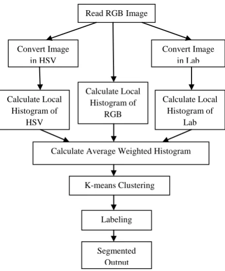
4. ARCHITECTURE AND ALGORIITHM

(2)

[image:2.595.50.282.119.398.2]

four steps: conversion of image, calculate local histogram, calculate average weighted histogram, K-means Clustering and Labeling which is shown below.

Figure 1: Flow chart for the proposed approach.

4.1 Color Conversion

In order to use a good color space for a specific application, color conversion is needed between color spaces. Here conversion of image is essential for local histogram calculation. At first convert RGB into HSV image and the conversion formula is as follows:

……… (1)

……..……… (2)

………. (3)

Another conversion performed that is RGB to Lab conversion. There are no simple formulas for conversion between RGB values and L*a*b* because the RGB color models are device dependent. The RGB values first need to transform to a specific absolute color space, such as RGB or adobe RGB. This adjustment will be device dependent, but the resulting data from the transform will be device independent, allowing data to be transformed to the CIE 1931 color space and then transformed into L*a*b*.

4.2 Local Histogram

global histogram which summarizes the entire image. A local histogram samples an area of particular interest laying within the image a spatial subset. In general the local histogram will be associated with the area of the image containing the subject. The histogram shows that the values are within an extremely narrow range. In contrast to the global histogram this local histogram tells that there is an examination of a nearly solid tone. Even without seeing the selection, one could guess the shape, location, and size of the selection.

This makes sense because the pixels are arranged randomly, so a large enough sample is representative of the distribution of pixels of the entire image. In this image there is no privileged view. A privileged view is a local view that offers information about whether it is in the global view. For this image any view should have the same histogram as the global as well as any other local view.

4.3 Average Weighted Histogram

During the histogram calculation, ten closest representative bins are found for each pixel. In CIEL*u*v* space, the distance between two colors (L1, u1, v1) and (L2, u2, v2) is calculated as

d = …… (4)

After ten closest bins found, weights are assigned to them which are inversely proportional to the distance between the pixel and bins. The total weight assigned to the ten bins, is equal to 1. The following equation shows how the weight is assigned to bin i (which is one of the ten closet bins):

……….. (5)

4.4 K-means Clustering

The K-Means is a nonhierarchical clustering technique that follows a simple procedure to classify a given data set through a certain number of K clusters that known as priori. The K-Means algorithm updates the space partition of the input data iteratively, where the elements of the data are exchanged between clusters based on a predefined metric (typically the Euclidian distance between the cluster centers and the vector under analysis) in order to satisfy the criteria of minimizing the variation within each cluster and maximizing the variation between the resulting K clusters. The algorithm is iterated until no elements are exchanged between clusters. This clustering algorithm, in its standard formulation consists mainly of four steps that are brieflydescribed below:

1. Initialization – generate the starting condition by defining the number of clusters and randomly select the initial cluster centers.

properly and are labeled with their mean colors. So the performance of our proposed segmentation method is better Read RGBImage

Convert Image in HSV

Convert Image in Lab

Calculate Local Histogram of

RGB Calculate Local

Histogram of HSV

Calculate Local Histogram of

Lab

Calculate Average Weighted Histogram

K-means Clustering

Labeling

(3)

2. Generate a new partition by assigning each data point to the nearest cluster center.

3. Recalculate the centers for clusters receiving new data points and for clusters losing data points.

4. Repeat the steps 2 and 3 until a distance convergence criterion is met.

As mentioned before, the aim of the K-Means is the minimization of an objective function that samples the closeness between the data points and the cluster centers and is calculated as follows:

|| xi(j)- cj||2 ……...(6)

[image:3.595.347.506.66.351.2]

5. LABELING AND SEGMENTATION

For every object in input k-means returns an index corresponding to a cluster. Label every pixel in the image with its cluster index. Objects in a binary image are pixels that are on i.e. set to the value 1, these pixels are considered to be the foreground. When you view a binary image, the foreground pixels appear white. Pixels that are off i.e. set to the value 0 are considered the background. When you view a binary image, the background pixels appear black. When a leading end of a run on an upper row in a binary mask which performs raster scan over a binary image is detected, a run label which was assigned to the same run when scanning a row preceding the current row by one row is read out and label diversion destination data is read from a concatenation table using the read run label as an address. A temporary label is determined by comparing a concatenated label, which indicates the minimum label value of the runs prior to the run on the upper row of which leading end is detected and adjacent to the run existing on the run on the lower row of the binary mask, with the diversion destination data read from the concatenation table. If one of them is 0, the other label data is issued as the temporary label. If both of them are 0, a new label is issued as the temporary label. If the compared label values are different from each and are not 0, the smaller label value is written into the concatenation table using the larger label value as the address. In the labeling process for a binary image data, a frequency of assignment of multiple labels to the same object is reduced, and thereby a load in a label integrating process is reduced. Finally we get the segmented image.

6. EXPERIMENTAL RESULT

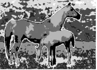
We have conducted our experiment based on color image. Different types of color images are available on the World Wide Web such as [11]. We have created cluster on color image to perform the experiment. Average weighted histograms are calculated and then k-means cluster is used for cluster. It can be observed from the experimental results that without a priori knowledge system could isolate the objects

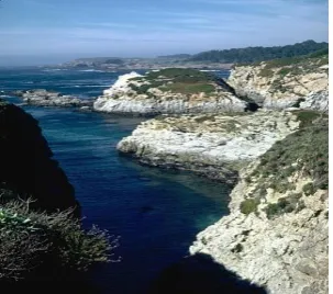
Figure 2: (a) Original Image

Figure 2: (b) K-means Clustering K=8

Figure 2: (c) Proposed method K=8

[image:3.595.353.505.73.190.2] [image:3.595.354.506.386.508.2] [image:3.595.354.506.540.674.2]

(4)

Figure 4: (a) Original Image

7 CONCLUSION

We have proposed a method for image segmentation. We have devised an algorithm for image segmentation for color image. The proposed algorithm will work on RGB, HSV and Lab color model. We merge these three different color models and finally perform the segmentation. Experimental results showed that this algorithm produce better result than the individual color model produces. We calculate the histogram of the image and then used K-means clustering algorithm for clustering. This algorithm produces better result in the point of finding the margin line of the objects. The comparison between different algorithm shows that proposed algorithm produces better output.

8 ACKNOWLEDGEMENTS

We are grateful to almighty, the most merciful that by his boundless grace we are able to publish our research work. We am expressing our hearty complements and indebted to my honorable supervisors for their affectionate guidance, instructions & informative suggestions, helpful assistance, patience & encouragement throughout the whole term which made us to the do this research. Finally, we are grateful to all of our friends, seniors, juniors and colleagues who have always been part of our life. Continuous inspiration and understanding of these individuals enabled us to cross the hurdles of our life.

9 REFERENCES

[1] Kanchan Deshmukh, Ganesh Shinde “Adaptive Color Image Segmentation Using Fuzzy Min-Max Clustering”

[2] James C. Tilton (PI), Giovanni Marchisio (Co-I) and Mihai Datcu (Co-I), "Knowledge Discovery and Data Mining Based on Hierarchical Segmentation of Image Data, " a research proposal submitted October 23, 2000 in response to NRA2-37143 from NASA's Information Systems Program.

[image:4.595.91.243.71.210.2] [image:4.595.348.512.72.190.2] [image:4.595.91.245.244.381.2] [image:4.595.85.250.566.685.2]

(5)

[5] K. Hohne, H. Fuchs, and S. Pizer, 3D Imaging in Medicine: Algorithms, Systems, Applications. Berlin, Germany: Springer-Verlag, 1990

[6] M. Bomans, K. Hohne, U. Tiede, and M. Riemer, “3-D segmentation of MR images of the head for 3-D display,” IEEE Trans. Med. Imag., vol. 9, pp. 253–277, June 1990.

[7] P. Willemin, T. Reed, and M. Kunt, “Image sequence coding by split and merge,” IEEE Trans.Commun., vol. 39, pp. 1845–1855, Dec. 1991.

[8] F. D. Natale, G. Desoli, D. Giusto, and G. Vernazza, “Polynomial approximation and vector quantization: A

region-based integration,” IEEE Trans. Commun., vol. 43, 1995

[9] K.S.Fu, J.K.Mui,”A Survey on image segmentation”. Pattern Recognition.