Numerical Solution of
n
-th Order Fuzzy Linear
Differential Equations by Homotopy Perturbation Method
Smita Tapaswini
Department of Mathematics, National Institute of Technology, Rourkela
Odisha - 769 008, India
S. Chakraverty
Department of Mathematics, National Institute of Technology, Rourkela
Odisha - 769 008, India
ABSTRACT
This paper targets to investigate the numerical solution of n -th order fuzzy differential equations wi-th fuzzy environment using Homotopy Perturbation Method (HPM). Triangular fuzzy convex normalized sets are used for the fuzzy parameter and variables. Obtained results are compared with the existing solution depicted in term of plots to show the efficiency of the applied method.
Keywords
n-th order fuzzy linear differential equations, Fuzzy Number, Triangular Fuzzy Number, Homotopy Perturbation Method (HPM).1.
INTRODUCTION
Theory of fuzzy differential equations plays an important role in modeling of science and engineering problems because this theory represents a natural way to model dynamical systems under uncertainty. There exist a large number of papers dealing with fuzzy differential equations and its applications in the open literatures. Some of are reviewed and cited here for better understanding of the present analysis. Chang and Zadeh [15] first introduced the concept of a fuzzy derivative, followed by Dubois and Prade [16] who defined and used the extension principle in their approach. The fuzzy differential equation and fuzzy initial value problems are studied by Kaleva [28, 29] and Seikkala [36]. Various numerical methods for solving fuzzy differential equations are introduced in [1, 2, 6, 31, 32, 37]. Very recently Tapaswini and Chakraverty [37] have proposed a new method to solve fuzzy initial value problem. Bede [11] described the exact solutions of fuzzy differential equations in his note in an excellent way. Buckley and Feurin [14] applied two analytical methods for solving n-th order linear differential equations with fuzzy initial conditions. Similarly many authors studied various other methods to solve n-th order fuzzy differential equations in [3, 4, 5, 7, 26]. Based on the idea of collocation method Allahviranloo et al. [5] investigated the numerical solution of n-th order fuzzy differential equations. Abbasbandy et al. [3] applied Runge-Kutta method for the numerical solution of n-th order fuzzy differential equations. The analytical method (eigenvalue-eigenvector method) for n-th order fuzzy differential equations with fuzzy initial value is also discussed by Allahviranloo et al. [7]. Abbasbandy et al. [4] and Jafari et al. [26] used variational iteration method for solving n-th order fuzzy differential equations recently. Besides the above approaches Homotopy Perturbation Method (HPM) is also found to be a powerful tool for solving the fuzzy differential equations. The HPM was first developed by He [20, 21] and many authors applied this method to solve various linear and non-linear differential equations of scientific and engineering problems. The solution is considered as the sum of infinite series, which converges rapidly to accurate solutions. In the homotopy technique (in topology), a homotopy is constructed with an embedding
parameter which is considered as a "small parameter". Very recently HPM has been applied to a wide class of physical problems [10, 12, 13, 17, 22, 23, 24, 25, 30, 33, 34, 39, 40, 41, 42, 43]. In these papers the parameters and variables are considered as crisp (exact). Few researchers have also investigated the solution of fuzzy differential equations using HPM [8, 9, 18, 38]. Allahviranloo et al. [8, 9] applied homotopy perturbation method (HPM) to solve fuzzy Fredholm integral equations and fuzzy Volterra integral equations. Numerical solution of fuzzy initial value problems under generalized differentiability by HPM is studied by Ghanbari [18]. The example problems solved in [18] only consider the positive coefficients of the fuzzy differential equations. Also, the author did not described how to tackle the n-th order fuzzy differential equations by using HPM. Recently, Tapaswini and Chakraverty [38] used HPM for solving fuzzy quadratic Riccati differential equations. As regards in the present analysis, HPM is used to handle the numerical solution of n-th order fuzzy differential equations with fuzzy initial conditions respectively. Here the exact solutions of the respective systems are also found by the authors for the comparison. In the following sections preliminaries are first given. Next, numerical implementation of HPM for n-th order fuzzy differential equations with fuzzy initial conditions is discussed. Lastly numerical examples and conclusions are given.
2.
PRELIMINARIES
In this section, we present some notations, definitions and preliminaries which are used further in this paper [19, 27, 35, 44].
Definition 2.1. Fuzzy number
A fuzzy number U~ is convex normalised fuzzy set U~ of the real line R such that
} ], 1 , 0 [ : ) (
{U~ x R xR
where, U~ is called the membership function of the fuzzy set and it is piecewise continuous.
Definition 2.2. Triangular fuzzy number
A triangular fuzzy number U~ is a convex normalized fuzzy setU~ of the real line R such that
i. There exists exactly one x0R with U~(x0)1 (
x
0is called the mean value of U~), where U~ is called the membership function of the fuzzy set.ii. U~(x) is piecewise continuous.
Let us consider an arbitrary triangular fuzzy number )
, , ( ~
c b a
c x c x b b c x c b x a a b a x a x x U , 0 , , , 0 ) ( ~
Any arbitrary triangular fuzzy number U~(a,b,c) can be represented with an ordered pair of functions through rcut approach viz. [u(r),u(r)][(ba)ra,(cb)rc] where, r[0,1].
For the triangular fuzzy numbers the left and right bound of the fuzzy numbers satisfies the following requirements i. u(r) is a bounded left continuous non-decreasing
function over [0, 1].
ii. u(r) is a bounded right continuous non-increasing function over [0, 1].
iii. u(r)u(r),0r1.
Definition 2.3. Fuzzy arithmetic
For any two arbitrary fuzzy number~x[x(r),x(r)], )]
( ), ( [ ~ y r y r
y and scalar k, the fuzzy arithmetic is defined as follows,
i. x~~yif and only if x(r)y(r)and x(r)y(r) ii. ~x~y[x(r)y(r),x(r)y(r)]
iii.
) ( ) ( ), ( ) ( ), ( ) ( ), ( ) ( max , ) ( ) ( ), ( ) ( ), ( ) ( ), ( ) ( min ~ ~ r y r x r y r x r y r x r y r x r y r x r y r x r y r x r y r x y x iv. 0 )], ( ), ( [ 0 )], ( ), ( [ ~ k r x k r x k k r x k r x k x k
Lemma 2.1. [11] If u~(t)(x(t),y(t),z(t)) is a fuzzy triangular number valued function and if u~ is Hukuhara differentiable, then u~(x,y,z). By using this property, we intend to solve the fuzzy initial value problem
0 0) ~
( ~ ) ~ , ( ~ x t x x t f x
with,x~ (x ,xc,x )R,x~(t)(u,uc,u)R 0 0 0 0 and
)). , , , ( ), , , , ( ), , , , ( ( )) , , ( , ( , ,: 0 0
u u u t f u u u t f u u u t f u u u t f R R a t t f c c c c c
We can translate this into the following system of ordinary differential equations as below:
0 ) 0 ( , ) 0 ( , ) 0 ( ) , , , ( ) , , , ( ), , , , ( 0
0 u x u x
x u u u u t f u u u u t f u u u u t f u c c c c c c c (1)
3.
HPM FOR
N-TH ORDER FDES
Consider the following n-th fuzzy differential equation ] 1 , 0 [ , 0 )) ( ~ , ), ( ' ' ~ ), ( ' ~ ), ( ~ , ( ) ( ~( ) ( ) t t y t y t y t y t f t
y n n (2)
with initial conditions
. 1 , , 2 , 1 , 0 )), ( ), ( ( ) 0 (
~y() g r k r i n
i i
i
By homotopy perturbation method [20, 21], we construct a simple homotopy as
~ () (,~(),~(),~(), ,~ ())
0, ~) 1
( p y(n)py(n) t f t y t yt yt y(n) t (3) or
(,~(),~(),~(), ,~ ())
0. )(
~y(n) t p f t y t yt yt y(n)t
(4) where, p[0,1] is an embedding parameter.
For p0, we obtain
, 0 ) ( ~( ) t y n from equation (3) and for p1,
0 )) ( ~ , ), ( ~ ), ( ~ ), ( ~ , ( ) (
~y(n) t f t y t yt yt y(n)t .
In topology, this is called deformation.
) ( ~( )
t
yn and ~y(n)(t)f(t,~y(t),~y(t),~y(t),,y~(n)(t)) are called homotopic.
Acording to HPM, we can assume that the solution of equation (3) or (4) can be expressed as a series in p.
~() ~() ~() ~() ) ( ~ 3 3 2 2 1
0t py t p y t p y t
y t
y (5)
when p1, equation (3) or (4) corresponds to equations (2) and (5) becomes the approximate solution of equation (2), i.e.,
~() ~() ~ () ~() ) ( ~ 3 2 1
0t y t y t y t
y t
y (6)
This is the approximate solution to equation (2). In most cases the series equation (6) is a convergent one which leads to the exact solution of equation (2). One can take the closed form or truncate the series for obtaining approximate solutions.
4.
NUMERICAL IMPLEMENTATION
OF THE METHOD
In this section we present the homotopy perturbation method for solving linear fuzzy differential equations
Example 1. [5] Let us consider the electrical circuit, where h
L1 , R2, C0.25f and E(t)20cost.If Qis the charge on the capacitor at time t0,then
cos 50 ) ( 4 ) ( ' ~ 2 ) ( ' ' ~ t t Q t Q t
Q (7)
subject to the initial conditions ), 6 , 4 ( ) 0 ( ~ r r
Q Q~(0)(r,2r). We have obtained the exact fuzzy solution as
) sin( 13 100 ) cos( 13 150 3 sin 13 250 2 8 3 1 3 cos 13 150 6 ) ; ( ) sin( 13 100 ) cos( 13 150 3 sin 13 250 4 2 3 1 3 cos 13 150 4 ) ; ( t t t r t r e r t Q t t t r t r e r t Q t t
The general terms of the equation cos 50 ) ( 4 ) ( ' 2 ) ( '
' t Q t Qt t
Q
cos 50 ) ( 4 ) ( ' 2 ) ( '
' t Q t Q t t
Q
Using HPM, we have the series solution as follows , ) 4 ( ) ; (
0t r r rt
q
, ) 2 ( ) 6 ( ) ; (
0t r r rt
q
, 1 ) cos( 3 2 ) 8 3 ( ) ;
( 2 3
1 t r r t rt t
q , 1 ) cos( 3 ) 2 ( 2 ) 3 14 ( ) ; ( 3 2
1 t
, 4 2 ) cos( 4 ) sin( 2 15 2 3 ) 4 8 ( 2 3 16 2 ) ; ( 5 4 3 2 2 t t t t r t r t r t r t q , 4 2 ) cos( 4 ) sin( 2 15 ) 2 4 ( 3 ) 4 16 ( 2 3 28 2 ) ; ( 5 4 3 2 2 t t t t r t r t r t r t q
and so on. The third term approximate solution for equation (7) is given by
[image:3.595.312.549.72.388.2] 4 2 ) cos( 4 ) sin( 2 15 2 3 ) 4 8 ( 2 3 16 2 1 ) cos( 3 2 ) 8 3 ( ) 4 ( ) ; ( 5 4 3 2 3 2 t t t t r t r t r t t rt t r rt r r t q 4 2 ) cos( 4 ) sin( 2 15 ) 2 4 ( 3 ) 4 16 ( 2 3 28 2 1 ) cos( 3 ) 2 ( 2 ) 3 14 ( ) 2 ( ) 6 ( ) ; ( 5 4 3 2 3 2 t t t t r t r t r t t t r t r t r r r t q
Fig 1: Fuzzy solution of the HPM for n=3.
Obtained results by the HPM for third order approximation and numerical solution of [5] are compared with the exact solution in Table 1 for t = 0.001. Moreover the HPM solution plot is given in Figure 1.
Example 2.[5]Let us consider another second order fuzzy linear differential equation
] 1 , 0 [ , 0 4 ' ~ 4 ''
~ y y t
y (8)
subject to the initial conditions ), 4 , 2 ( ) 0 (
~y r r y~(0)(5r ,7r)
This problem has also been solved by Allahviranloo et al. [5]. The authors [5] have studied both numerical solution as collocation type method and exact solution. It may be mentioned that the exact solution obtained by [5] does not satisfy the differential equation. So, here we have obtained the exact fuzzy solution for this differential equation by using the method of [11]. The same may be given as
t t e e t r r t
Y( ; )( 1)(13) 2 3 2
t t e e t r r t
Y( ; )(1 )(13) 2 3 2
Now, using HPM method, we get the four term approximate solution for equation (8) as follows:
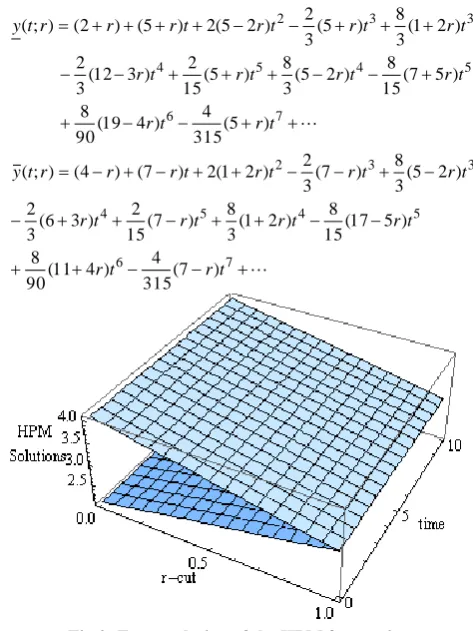
7 6 5 4 5 4 3 3 2 7 6 5 4 5 4 3 3 2 ) 7 ( 315 4 ) 4 11 ( 90 8 ) 5 17 ( 15 8 ) 2 1 ( 3 8 ) 7 ( 15 2 ) 3 6 ( 3 2 ) 2 5 ( 3 8 ) 7 ( 3 2 ) 2 1 ( 2 ) 7 ( ) 4 ( ) ; ( ) 5 ( 315 4 ) 4 19 ( 90 8 ) 5 7 ( 15 8 ) 2 5 ( 3 8 ) 5 ( 15 2 ) 3 12 ( 3 2 ) 2 1 ( 3 8 ) 5 ( 3 2 ) 2 5 ( 2 ) 5 ( ) 2 ( ) ; ( t r t r t r t r t r t r t r t r t r t r r r t y t r t r t r t r t r t r t r t r t r t r r r t y
Fig 2: Fuzzy solution of the HPM for n=4.
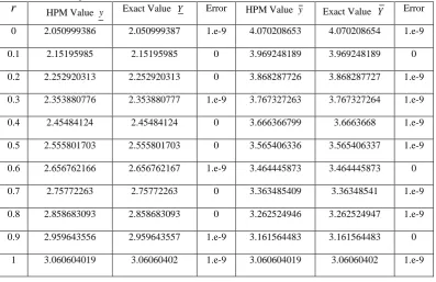
The exact, numerical solution obtained by [5] and present solution using HPM are tabulated in Table 2 for t = 0:01. Errors obtained are also incorporated in this table. By looking into the results, one may conclude that the solution obtained by HPM is the same as that of the exact solution. The solution plot is given in Figure 2.
Example 3: [4] Let us consider the following fourth order fuzzy linear differential equation
] 1 , 0 [ , ~
~y(4)y t
(9)
subject to the initial conditions ), 1 , 1 ( ) 0 (
~y r r y~(0)(r1,1r), ~y(0)(r1,1r) and ~y(0)(r1,1r)
The exact fuzzy solution as given in [4] is, t
e r r t
Y( ; )( 1) t e r r t
Y( ; )(1 )
Applying the same procedure as in example (1)-(2), we get the approximate solution for equation (9) as
! 7 ! 6 ! 5 ! 4 ! 3 ! 2 1 ) 1 ( ) ; ( 7 6 5 4 3 2 0 t t t t t t t r r t y ! 7 ! 6 ! 5 ! 4 ! 3 ! 2 1 ) 1 ( ) ; ( 7 6 5 4 3 2 0 t t t t t t t r r t y
leading to the closed form
t t e r r t y e r r t y ) 1 ( ) ; ( ) 1 ( ) ; (
[image:3.595.54.287.209.505.2]solved by Abbasbandy et al. [4] using variational iteration method.
It may be noted that the closed form of the first order approximation of HPM will exactly be same as the exact
[image:4.595.100.497.144.400.2]solution. Where, as in [4] it takes 10th iteration to get the approximate solution. The corresponding plot of the solution using HPM is given in Figure 3.
Table 1: Comparison of the HPM and exact solutions for n=4 with different r and t0.001.
r HPM Value q Exact Value Q Error HPM Value q Exact Value Q Error 0 3.999992505 4.000016989 2.4e-5 6.001986508 6.002010991 2.4e-5
0.1 4.100092205 4.100116689 2.4e-5 5.901886808 5.901911291 2.4e-5
0.2 4.200191905 4.200216389 2.4e-5 5.801787107 5.801811591 2.4e-5
0.3 4.300291605 4.300316089 2.4e-5 5.701687407 5.701711891 2.4e-5
0.4 4.400391306 4.400415789 2.4e-5 5.601587707 5.601612191 2.4e-5
0.5 4.500491006 4.500515489 2.4e-5 5.501488007 5.501512491 2.4e-5
0.6 4.600590706 4.600615189 2.4e-5 5.401388307 5.401412791 2.4e-5
0.7 4.700690406 4.70071489 2.4e-5 5.301288607 5.30131309 2.4e-5
0.8 4.800790106 4.80081459 2.4e-5 5.201188907 5.20121339 2.4e-5
0.9 4.900889806 4.90091429 2.4e-5 5.101089206 5.10111369 2.4e-5
1 5.000989506 5.00101399 2.4e-5 5.000989506 5.00101399 2.4e-5
Table 2: Comparison of the HPM and exact solutions for n=4 with different r and t0.01.
r
HPM Value y Exact Value Y Error HPM Value y Exact Value Y Error 0 2.050999386 2.050999387 1.e-9 4.070208653 4.070208654 1.e-90.1 2.15195985 2.15195985 0 3.969248189 3.969248189 0
0.2 2.252920313 2.252920313 0 3.868287726 3.868287727 1.e-9
0.3 2.353880776 2.353880777 1.e-9 3.767327263 3.767327264 1.e-9
0.4 2.45484124 2.45484124 0 3.666366799 3.6663668 1.e-9
0.5 2.555801703 2.555801703 0 3.565406336 3.565406337 1.e-9
0.6 2.656762166 2.656762167 1.e-9 3.464445873 3.464445873 0
0.7 2.75772263 2.75772263 0 3.363485409 3.36348541 1.e-9
0.8 2.858683093 2.858683093 0 3.262524946 3.262524947 1.e-9
0.9 2.959643556 2.959643557 1.e-9 3.161564483 3.161564483 0
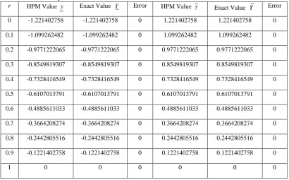
[image:4.595.100.498.438.695.2]Table 3: Comparison of the HPM and exact solutions for n=4 with different r andt0.2.
r HPM Value y Exact Value Y Error HPM Value y Exact Value Y Error
0 -1.221402758 -1.221402758 0 1.221402758 1.221402758 0
0.1 -1.099262482 -1.099262482 0 1.099262482 1.099262482 0
0.2 -0.9771222065 -0.9771222065 0 0.9771222065 0.9771222065 0
0.3 -0.8549819307 -0.8549819307 0 0.8549819307 0.8549819307 0
0.4 -0.7328416549 -0.7328416549 0 0.7328416549 0.7328416549 0
0.5 -0.6107013791 -0.6107013791 0 0.6107013791 0.6107013791 0
0.6 -0.4885611033 -0.4885611033 0 0.4885611033 0.4885611033 0
0.7 -0.3664208274 -0.3664208274 0 0.3664208274 0.3664208274 0
0.8 -0.2442805516 -0.2442805516 0 0.2442805516 0.2442805516 0
0.9 -0.1221402758 -0.1221402758 0 0.1221402758 0.1221402758 0
[image:5.595.49.302.88.527.2]1 0 0 0 0 0 0
Fig 3: Fuzzy solution of the HPM for n=4.
5. CONCLUSIONS
In this paper, HPM has been successful applied to find the solution of n-th order fuzzy differential equations. The solution obtained by HPM is an infinite series with appropriate initial condition, which in turn be expressed in a closed form i.e the exact solution. The result shows that the HPM is a powerful mathematical tool to solve n-th fuzzy differential equation. The solutions obtained are shown graphically.
6.
ACKNOWLEDGEMENT
The first author would like to thank the UGC, Government of India, for financial support under Rajiv Gandhi National Fellowship (RGNF).
7.
REFERENCES
[1] Abbasbandy S., Allahviranloo T., Numerical solutions of fuzzy differential equations by taylor method, Computational Methods in Applied Mathematics 2, 113– 124, (2002).
[2] Abbasbandy S., Allahviranloo T., Lopez-Pouso O., Nieto J.J., Numerical methods for fuzzy differential inclusions, Computer and Mathematics With Applications 48, 1633– 1641 (2004).
[3] Abbasbandy S., Allahviranloo T., Darabi P., Numerical solution of n-order fuzzy differential equations by runge-kutta method, Mathematical and Computational Applications, 16, 935-946 (2011).
[4] Abbasbandy S., Allahviranloo T., Darabi P., O. Sedaghatfar, Variational Iteration method for solving n-th order fuzzy differential equations, Man-thematical and Computational Applications, 4,819-829 (2011).
[5] Allahviranloo T., Ahmady E., Ahmady N., N-th order fuzzy linear differential equations, Information science, 178, 1309-1324 (2008).
[6] Allahviranloo T., Ahmady N., Ahmady E., Numerical solution of fuzzy differential equations by predictor– corrector method, Information Sciences 177/7, 1633– 1647 (2007).
[7] Allahviranloo T., Ahmady N., Ahmady E., A method for solving n-th order fuzzy linear differential equations, Comput. Math. Appl 86, 730-742 (2009).
[8] Allahviranloo T., Hashemzehi S., The Homotopy Perturbation Method for Fuzzy Fredholm Integral Equations, Journal of Applied Mathematics, Islamic Azad University of Lahijan, 5, 1-12 (2008).
[9] Allahviranloo T., Khezerloo M., Ghanbari M. and Khezerloo S., The Homotopy Perturbation Method for Fuzzy Volterra Integral Equations, international journal of computational cognition 8,31-37 (2010).
[11] Bede B., “Note on numerical solutions of fuzzy differential equations by predictor-corrector method”, Information Sciences, 178, 1917-1922 (2008).
[12] Biazar J., Ghazvini H., Exact solutions for nonlinear Schrödinger equations by He’s homotopy perturbation method, Physics Letters A 366, 79–84 (2007).
[13] iazar J., Hosseini K., Gholamin P., Homotopy perturbation method Fokker-Plank equation, International Mathematical Forum, 19, 945-954, (2008).
[14] Buckley J. J., Feuring T., Fuzzy initial value problem for Nth-order linear differential equations, Fuzzy Sets and Systems 121, 247-255 (2001).
[15] Chang S. L. and Zadeh L.A., On fuzzy mapping and control, IEEE Transaction on Systems Man and Cybernetics, 2, 30-34 (1972).
[16] Dubois D. and Prade H., Towards fuzzy differential calculus: Part 3, differentiation, Fuzzy Sets and Systems, 8, 225-233 (1982).
[17] Ganji D. D., The applications of He’s homotopy perturbation method to nonlinear equation arising in heat transfer, Physics letter A, 335, 337-341 (2006).
[18] Ghanbari M., Numerical solution of fuzzy initial value problems under generalized differentiability by HPM, Int. J. Industrial Mathematics 1, 19-39 (2009).
[19] Hanss M Applied Fuzzy Arithmetic: An Introduction with Engineering Applications. Springer-Verlag, Berlin, 2005
[20] He J. H., Homotopy perturbation technique, Computer Methods in Applied Mechanics and Engineering, 178, 257-262 (1999)
[21] He J. H., A coupling method of homotopy technique and a perturbation technique for nonlinear problems, International Journal of Non-linear Mechanics, 35, 37-43 (2000).
[22] He J. H.,The homotopy perturbation method for nonlinear oscillators with discontinuities, Applied Mathematics and Computation 151, 287–292 (2004)
[23] He J. H., Application of homotopy perturbation method to nonlinear wave equations, Chaos, Solitons and Fractals 26, 695–700 (2005).
[24] He J. H., Homotopy perturbation method for solving boundary value problems, Physics Letters A 350, 87–88 (2006).
[25] Hosseinnia S. H., Ranjbar A., Ganji D. D., Soltani H., Ghasemi J., Homotopy perturbation based linearization of nonlinear heat transfer dynamic, Journal of Applied Mathematics and Computing 29: 163–176 (2009).
[26] Jafari H., Saeidy M., Baleanu D., The Variational Iteration method for solving n-th order fuzzy differential equations, central European Journal of Physics, 10, 76-85 (2012).
[27] Jaulin L., Kieffer M., Didri O. t, and Walter E., Applied Interval Analysis, Springer, (2001).
[28] Kaleva O., Fuzzy differential equations, Fuzzy Sets and Systems, 24, 301-317 (1987).
[29] Kaleva O., The Cauchy problem for fuzzy differential equations, Fuzzy Sets and Systems, 35, 389-396 (1990).
[30] Khaki M., Ganji D. D., Analytical solutions of nano boundary layer flows by using he’s homotopy perturbation method, Mathematical and Computational Applications, 15, No. 5, 962-966, (2010).
[31] Ma M., Friedman M., and Kandel A., Numerical solutions of fuzzy differential equations, Fuzzy Sets and Systems, 105, 133-138 (1999) .
[32] Mikaeilvand N., Khakrangin S., Solving fuzzy partial differential equations by fuzzy two-dimensional differential transform method, Neural Computing and Application 21, S307–S312, (2012).
[33] Nave1 O., Lehavi Y., Goldshtein V. and Ajadi S., Application of the Homotopy Perturbation Method (HPM) and the Homotopy Analysis Method (HAM) to the Problem of the Thermal Explosion in a Radiation Gas with Polydisperse Fuel Spray, Applied & Computational Mathematics, 2012, 1:4.
[34] Rafie M. , Ganji D. D., Explicit solutions of Helmholtz equation and fifth order KdV equation using homotopy perturbation method, International journal of Nonlinear Sciences and Numerical simulation, 7,321-328 (2006).
[35] Ross T. J., Fuzzy logic with engineering applications. Wiley Student Edition, 2007.
[36] Seikkala S., On the fuzzy initial value problem, Fuzzy Sets and Systems, 24, 319-330 (1987).
[37] Tapaswini Smita and Chakraverty S, A New Approach to Fuzzy Initial Value Problem by Improved Euler Method. International J Fuzzy Inf Eng 4, 293-312 (2012).
[38] Tapaswini Smita and Chakraverty S., Homotopy perturbation method for solving fuzzy quadratic Riccati differential equations, 39th Annual conference of Orissa Mathematical Society and National seminar on cryptography, VIVTECH, Bhubaneswar, Odisha, 4th -5th February, (2012).
[39] Thiagarajan S., Meena A., Anitha S., Rajendran L., Analytical expression of the steady-state catalytic current of mediated bioelectrocatalysis and the application of He’s Homotopy perturbation method, Journal of Mathematical Chemistry, Journal of Mathematical Chemistry 49, 1727–1740 (2011).
[40] Vanani S. K., Soleymani F., Application of the Homotopy Perturbation Method to the Burgers Equation with Delay, Chin.phys.lett. 29, 030202 (2012)
[41] Zare M., Jalili O. and Delshadmanesh M, Two binary stars gravitational waves: homotopy perturbation method, Indian J Phys, 86, 855–858 (2012).
[42] Zedan H. A. and Tantawy S. Sh., Solution of Davey– Stewartson Equations by Homotopy Perturbation Method, Computational Mathematics and Mathematical Physics, 49, 1382–1388 (2009).
[43] Zhang B., Liu Zheng-Rong, Jian-Feng Mao, Approximate explicit solution of Camassa-Holm equation by He’s homotopy perturbation method, J Appl Math Comput 31: 239–246 (2009) .