The Demand for Money in Greece 1962 to 1998

Munich Personal RePEc Archive

The Demand for Money in Greece 1962

to 1998

Loizos, Konstantinos and Thompson, John

SOAS, University of London, Liverpool Business School

January 2001

THE DEMAND FOR MONEY IN GREECE 1962 TO 1998

by

Konstantinos Loizos (SOAS, University of London)

and

John Thompson

(Liverpool Business School)

The authors wish to thank Professor K Holden, Liverpool Business School, for his helpful comments and suggestions in the preparation of this paper but we would like to emphasise that any errors remaining the paper are entirely our responsibility.

January 2001

ABSTRACT

The paper examines the demand for narrow money in Greece over the period 1962 to 1998. The data is tested to examine the order of integration. Estimation of the demand function follows the two step methodology. The first step entails the specification of the long run equilibrium relationship between real narrow money, the index for industrial production (a proxy for real income), an interest rate and the rate of inflation through the estimation of the cointegrating vector by the Johansen technique. The second step involves an Error Correction Equation being estimated to provide the short-run dynamics. Finally the model is simulated to see how well it tracks the actual values of the dependent variable.

1

The demand for money assumes an important component of

theoretical models of any economy and as such has been the subject

of many studies for a wide variety of countries. In section 1 of this

paper we start by providing a brief review of the financial history of

Greece and a summary of what we consider to be key studies of the

demand for money in Greece. A discussion of the nature of the data is

presented in section 2. The empirical results are discussed in sections

3 and 4. The model is tested for its simulation properties in section 5

and our conclusions in section 6.

The Greek financial system was heavily regulated during the post-war

period until the mid-eighties. Major characteristics of this system are

the administratively set interest rates, the compulsory channeling of a

proportion of bank reserves into various uses and sectors indicated by

the authorities, the financial support of the government at

below-market rates and the control of foreign exchange transactions. Given

that banks were the dominant financial intermediaries while capital

market was underdeveloped, investment opportunities were heavily

dependent to the government priorities.

However, this picture altered, during the late eighties and nineties,

through a process of financial liberalization that aimed to restore

market conditions throughout the system. Important steps included

the gradual deregulation of bank lending and borrowing rates, the

removal of credit restrictions imposed on commercial banks, the

resumption of Treasury Bills sales directly to the public in 1985 and

the abolition of controls in capital movements in 1994. In 1994, the

government also lost its privileged access to the Central Bank while its

With respect to the formulation of the demand for money function the

following points are important:

a) The underdevelopment of capital market along with the

regulated nature of the system for most of the period

indicates the significant role of real assets and hence of

inflation (their rate of return) as a determinant of money

demand.

b) The constrained opportunities for financial investments

restrict the choice of a representative rate of return on

financial assets as a rate of interest on bank deposits.

c) Finally, the transition period from regulation to

liberalization during the last third of the estimation period

raises the interesting question of the stability of demand

for money along with the problem of the appropriate

independent variables in this function.

Figure 1 shows the growth of M1 during this period and, whilst the

financial liberalisation discussed above must have affected the

behaviour of the money supply, the pattern in Chart 1 shows no

sudden changes or jumps in the time pattern of the growth of nominal

narrow money supply. We have therefore not included any dummy

variables to represent any of the measures discussed above1_{. In}

general our approach will be a compromise between the various

traditions in the theoretical development of the demand for money and

will include as explanatory variables the rate of inflation, the level of

real GDP (y) and a representative rate of interest (r). Consequently we

include both the return on financial assets (i.e. the representative rate

of interest) and also the return on real assets {represented by the

expected rate of inflation (infl)} as well as the demand for transaction

purposes. This formulation is summarised below:

1

M/P = F(y, r, infl) with F1 > 0, F2 and F3 < 0 (1)

We now review briefly the existing literature on the demand for money

in Greece. These include Apostolou and Varelas [1987], Alexakis

[1980], Brissimis and Leventakis [1981,1983 and 1985], Ericsson and

Sharma [1998], Himarios [1983, 1986 and 1987], Palaiologos [1982],

Panayotopoulos [1983 and 1984], Prodromidis [1984] and Tavlas

[1987]. In order to simplify the discussion, we focus on just four

studies, which indicate the flavour of the existing literature. These

studies can usefully be categorised into those, which use annual data

e.g. Himarios [1986], Apostolou and Varelas [1987], and those, which

use quarterly data such as Psaradakis [1993], Ericsson and Sharma

[1998]. Himarios [1986] employs the partial adjustment hypothesis to

explain the demand for M1 and M2. According to Himarios’ results,

the demand for m12 is better explained by current income and a

short-term interest rate. The coefficient for inflation is insignificant at the

5% level. Despite the administrative nature of interest rates,

substitution between demand for m1 and financial assets is indicated

by the significance of the interest rate coefficient at the 5% level.

Demand for m2 is best explained by permanent income and expected

inflation with strongly significant coefficients whilst interest rates

coefficients are insignificant at the 5% level in most equations. Finally,

autocorrelation is removed when the lagged dependent variable enters

the functions, which may indicate the existence of adjustment costs. A

similar approach (i.e. the Partial Adjustment Hypothesis) was followed

by Apostolou and Varelas [1987], who also incorporate the level of

current income as an explanatory variable in their equation. Their

results suggest that the three variables (i.e. income, interest rate and

inflation) are all relevant to the explanation of the demand for money

in Greece. These results were troubled by the presence of

significance bounds were approached. In the case of the squares the lower boundary was approached only for the period 1979 to 1983.

2

autocorrelation, which was removed by the Cochrane-Orcutt method

of estimation.

The second two studies using quarterly data also use more

sophisticated techniques. Psaradakis [1993]3 _{estimates a vector}

autoregression model (VAR) for the period 1960 quarter1 to 1989

quarter 1. The estimated model found a role for interest rates,

inflation and income in the determination of the demand for money.

Whereas the previous studies mentioned all concentrated on M1 or

M2, Ericcson and Sharma [1998] examined the stability of broad

money M3 over the period 1975 to 1994. They found a role for income,

various interest rates and inflation.

As noted earlier, we estimate an equation of the following form to

represent the demand for M1:

(M/P)D = fN(y, r, infl) (1)

where M = M1 (i.e. narrow money), P = the price level, y real income, r

a representative rate of interest and infl the actual rate of inflation

used as a proxy for the expected rate o inflation. All the variables will

be specified in logarithmic form. The exact definition of the variables is

discussed in the following section.

2

Quarterly data on Gross Domestic Product for Greece are not available

before 1975 so it is necessary to use some proxy for income in the

demand for money function. As noted earlier Psaradakis [1993] used a

univariate time series model to construct a synthetic series of national

income on a quarterly basis. We have adopted a different approach by

using the index of industrial production as a surrogate for national

income. We acknowledge that use of the index of industrial production

3

represents just one sector (but a major one)4 _{of an economy but its}

value as a proxy is essentially an empirical matter. The correlation

coefficient for the natural logarithm values of annual data for GDP

deflated by the consumer price index and the index of industrial

production is 0.9653 for 1962 to 1997. We would therefore contend

that the index of industrial production is a good proxy for real GDP.

The specification of the other variables is less contentious. The rate of

interest adopted for the study is the 3 – 6 months’ time deposit rate

with commercial banks (lrs) and as such represents the return on the

closest substitute financial asset. The consumer price index (lp) is

used to denote the price level since this is the most widely published

index in Greece. In a similar manner the rate of inflation (infl) is the

first difference of the logarithm of the consumer price index. The

statistics were obtained from International Financial Statistics as

recorded by Datastream. Full details are shown in the appendix.

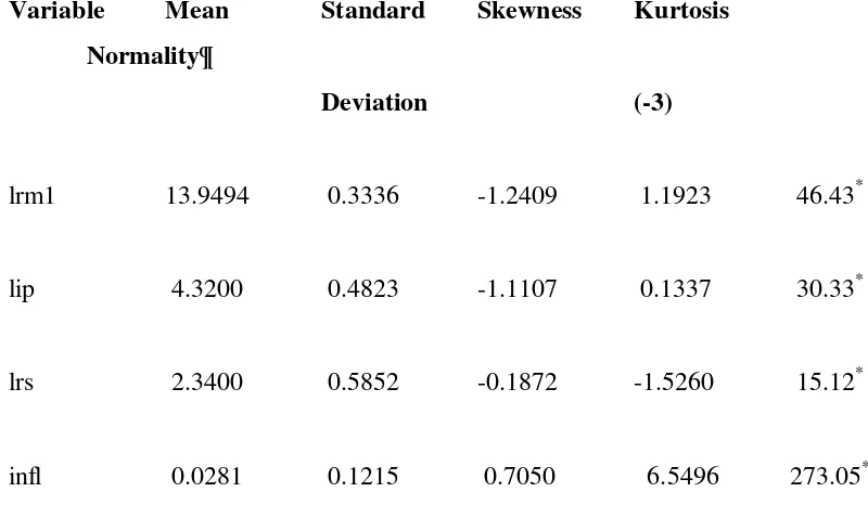
Descriptive statistics of the four variables of interest are shown in

Table 1. The first three variables show evidence of negative skewness

so that the distribution shows a longer tail to the left. As far as

kurtosis is concerned three variables (lrm1, lip and infl) show evidence

of positive kurtosis (i.e. leptokurtic) as compared with the normal

distribution i.e. the tails of the distribution are slimmer/longer than

that predicted by the normal curve. In the case of lrs, there is evidence

of fat or short tails (i.e. platykurtic). It would appear that none of the

variables are normally distributed and this is confirmed by the results

of the Bera-Jacques tests shown in the table.

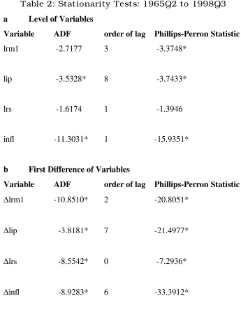
We now consider the order of integration of the variables5_{. Stationarity}

tests were carried out the variables (all in logarithmic form) real m1

(lrm1), the industrial production index (lip), the rate of interest (lrs)

4

However it is a fact that the empirical elasticities of the demand for money with respect to this index are not strictly comparable to those for GDP.

5

and inflation (infl) using Dickey-Fuller6 _{and Phillips-Perron}7 _{unit root}

tests. Augmented Dickey-Fuller (ADF) statistics were calculated with

lags up to 12 periods thus compressing the data into the period 1965

quarter 2 to 1998 quarter 3. Selection of the appropriate lag was

based on the information criteria provided by the Akaike (AIC),

Schwarz-Bayesian (SBC) and the Hannan-Quinn (HQC) statistics. In

the case of different recommendations provided by the criteria, greater

weight was afforded to the SBC and HQ statistics in view of the

tendency of the AIC statistic to overestimate the lag8_{. The equation}

implied by the selected lag was then tested for autocorrelation in the

residuals and in no case was the hypothesis of non-autocorrelated

residuals rejected. Tests were also carried out to ascertain if it was

appropriate to include a time trend in the ADF equation. In general

the hypothesis that the time trend was zero was not rejected9,10_{. The}

results are shown in Table 2.

The degree of integration is clear-cut in the case of lrs. The hypothesis

that the variable is stationary (i.e. I(1)) is rejected for levels but

accepted for first differences, suggesting that lrs is I(1). There is some

ambiguity concerning the results of the test for lrm1. The hypothesis

of stationarity is rejected by the ADF test but accepted by the

Phillips-Perron test. The hypothesis of stationarity is accepted for the first

differences of the variable. In contrast both lip and infl seem to be I(0)

with both the ADF and Phillips-Perron statistics indicating

stationarity. Both Psaradakis (1993) and Ericsson and Sharma (1998)

indicate the existence of unit Root for infl. Therefore, we propose

initially to consider both lip and infl as I(1). If the cointegrating vector

obtained under this assumption is statistically and theoretically

acceptable then it can be assumed that the results of the ADF tests for

6

See Dickey and Fuller [1981] 7

See Phillips and Peron [1988] 8

See Basçi and Zaman [1998] 9

The relevant critical values were obtained from Dickey and Fuller [1981]. 10

lip and infl are misleading. We discuss the estimation of equation (1)

in the following section.

3

The methodology adopted by us is a two step method using the

Johansen method (see for example Johansen [1988]) for estimation of

the long run, i.e. cointegrating, relationship between the variables. The

second step estimates the dynamic or short-run adjustment through

an error correction model (ECM)11_.

It is first of all necessary to examine whether the specific function

should include either (or both) a time trend and a constant. We tested

for the omission of the two variables individually and collectively. The

hypothesis that the coefficient on the time trend was zero was not

rejected at the 5% level. In contrast the hypothesis that the constant

was zero was rejected at the 5% level. Not unnaturally the joint

hypothesis that the coefficient on the time trend and the constant

were zero was rejected at the 5% level. These tests left the proposed

cointegrating equation including a constant but excluding a time

trend.

It was then necessary to decide on the order of the VAR. In line with

our earlier comments on the bias of the Akaike criterion we relied on

the Schwarz Bayesian criterion which suggested the order to be 4. We

then tested for the number of cointegrating vectors within the model.

The results of the tests are, to say the least, inconclusive. At the 5%

level of significance, the tests based on the maximal eigenvalue and

the trace both indicated 2 cointegrating vectors. In contrast to these

results, tests based on model selection criteria were contradictory with

the Akaike Information, the Schwarz Bayesian and the Hannan-Quinn

11

criteria suggesting the number of cointegrating vectors as 4, 3 and 3

respectively. We selected three as the number of cointegrating vectors

and their respective values are shown in Table 3.

Interpretation of estimated cointegrating vectors can be difficult but

the first two vectors appear to be defective since either the magnitude

or the sign of some of the coefficients do not accord with economic

theory. On the other hand, for the third vector, the signs of the

estimated coefficients are consistent with theory as indicated with

reference to equation 1. The selected cointegrating vector is therefore:

lrm1 = 11.072 + 0.814*lip – 0.272*lrs – 0.189*infl (2)

The long-run elasticities indicated in equation 2 seem quite sensible.

Both the interest and inflation elasticities are negative and less than 1

suggesting that the demand for real M1 is inelastic with respect to

these two variables. Little can be said about the elasticity with respect

to the index of industrial production because this variable is a proxy

for real GDP. It is instructive to compare elasticities with those

obtained in other studies. Examples are shown below:

rs infl

Present study -0.27 -0.19

Himarios [1986] -0.30 -0.11

Apostolu & Varleas [1987]

1960 – 1982 -0.16 -0.87

1969 – 1982 -0.26 -0.48

Psaradakis [1993] n/a -8.93

With the exception of the inflation elasticity obtained by Psaradakis,

our estimates are within the same broad range obtained by the other

studies.

In the next section we turn to discuss the dynamic structure of the

4

We use the general-to-specific approach starting off with the following

model12 _{of the ECM:}

∆lrm1 = α0 + Σβi∆lipt-i + Σγ∆lrst-i + Σδ∆inflt-i + λrest-I + α1SR1

+ α2SR2 + α3SR3 + εt (3)

where res refers to the residuals from the cointegrating equation, SR1,

SR2 and SR3 are seasonal dummy variables and ε is the error term.

The ECM was then simplified by a process of sequential elimination of

variables for which the coefficients were not statistically different from

zero at the 5% level of significance; i.e. we used the general to the

specific approach. The preferred ECM is:

∆lrm1 = 0.058 + 0.185*∆lipt-2 –0.146*∆rlst-3 – 0.749*∆infl – 0.450*∆inflt-1

-0.135*∆inflt-2 –0.249*rest-3 – 0.197*S1 (4)

Full details of the estimated equation are shown in Table 4. It is

worth noting at this stage that:

a) The ‘t’ values of the estimated coefficients indicate coefficients

which are significantly different from zero in six cases out of eight;

one further case is significant at the 10% level and the remaining

coefficient verges on significance at this latter level.

b) Lagging the residual variable 3 periods produced the coefficient

with the highest ‘t’ value for this variable,

c) Although three seasonal dummy variables were tried only one

proved significantly different from zero at the 5% level. The ‘F’ test

failed to reject the hypothesis that the coefficients on the variables

12

S2 and S3 were jointly zero. Consequently only S1 appears in the

preferred ECM.

d) The significance of the coefficient for the lagged residuals from the

cointegrating equation implies that the explanatory variables in the

long-run equation are, in fact, cointegrated.

The diagnostics reported in Table 4 suggest that equation (4) passed

the autocorrelation and heteroscedascity tests satisfactorily but failed

the normality test for the residuals. The most important consequence

of this failure is probably to render invalid significance tests in the

case of small samples. Given the number of observations in our

sample (142) we suggest that our significance tests are valid but we

note this defect in the preferred ECM.

Combination of equation (4) and equation (2) produces the final

equation (5) explaining the demand for M1 in Greece:

lrm1 = lrm1(-1) + 0.058 + 0.185*∆lipt-2 – 0.146*∆rlst-3 – 0.749*∆infl –

0.450*∆inflt-1 - 0.135*∆inflt-2 – 0.249*{lrm1t-3 –(11.072

+0.814*lipt-3 – 0.272lrst-3 – 0.189*infl)

–0.197*S1 (5)

We now move on to see how well the predictions from equation (5)

track the actual values of rm1.

5

We report the results of ex-post static and also dynamic simulation of

equation 5 over the period 1963 quarter 2 to 1993 quarter; i.e.

including four periods outside the estimation period13_{. The results are}

depicted in figures 2 and 3 with the area to the right of the dotted line

13

indicating post estimation-period simulations. The relevant diagnostic

statistics for the within estimation-period simulations are shown in

table 5.

A cursory glance at figure 2 suggests that the model tracks the

behaviour of LRM1 quite well. There appear to be no significant

departures from the observed behaviour of LRM1. This tends to

confirm our view that the model did not require the introduction of

dummy variables to allow for the various changes in the financial

environment.

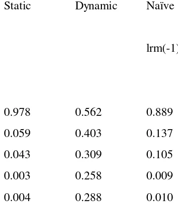
As far as the static simulation results are concerned, the satisfactory

quality of the model as far as tracking actual values of the log of the

real money supply is confirmed by the statistics shown in table 5. The

correlation coefficient between the simulated and actual values is

quite high and the various error statistics quite low. As a yardstick we

also obtained the same statistics for the naïve ‘no-change model’.

These are also shown in table 5 and, in every case are inferior to those

relevant to model predictions. The mean error for the model

simulation is also not significantly different from zero. This suggests

that the model is providing unbiased biased ‘in sample’ forecasts14_.

Dynamic simulations provide a much more (?excessively) rigorous test

of the model. Examination of chart 3 shows that the demand for

money was significantly under predicted for the period 1969 to 1986.

Outside this period however, the actual behaviour of lrm1 was well

tracked. These conclusions are reinforced by examination of the

statistics contained in Table 5. In every case, as would be expected,

the diagnostic statistics for the dynamic simulations are inferior to

both the ex-post static simulations and the naïve forecasts.

Furthermore the hypothesis that the mean error is zero is rejected at

the 5% level of significance. This is no doubt to the under prediction

which occurred in the period 1969 to 1986.

14

6 Conclusions

This paper raised the issue of the long-run equilibrium relationship of

demand for money and its short run dynamics, in the context of the

Greek economy during a period experiencing conflicting developments

in its real and financial sector. The function was estimated using a

method based on the Granger-Engle two step method. The Johansen

procedure that was implemented to obtain the long-run (equilibrium)

relationship while the short-run dynamics were obtained through

estimation of an ECM which gave significant and correctly signed error

correction terms. These results should confirm the existence of

long-run stable relationship between M1 and a three other variables, i.e. the

index of industrial production (lip, a proxy for national income), a

short rate of interest (lrs) and the rate of inflation (infl). Apart from the

failure of the normality test for the residuals, the preferred ECM was

satisfactorily estimated. Furthermore, the estimated elasticities

indicated the dependence of money demand on inflation both in the

long run and short run. Hence, the inclusion of inflation in the

function seems justified denoting that real assets were an important

alternative to money during that period.

Finally the model tested by simulated the final equation within the

sample period. Ex Post Static simulations provided evidence that the

final equation tracked the actual variables in a satisfactory manner.

The Ex Post Dynamic simulations, whilst providing inferior results to

the static simulations, were also reasonably satisfactory given the

Table 1: Descriptive Statistics: 1962Q1 to 1998Q3

Variable Mean Standard Skewness Kurtosis

Normality¶

Deviation (-3)

lrm1 13.9494 0.3336 -1.2409 1.1923 46.43*

lip 4.3200 0.4823 -1.1107 0.1337 30.33*

lrs 2.3400 0.5852 -0.1872 -1.5260 15.12*

infl 0.0281 0.1215 0.7050 6.5496 273.05*

Table 2: Stationarity Tests: 1965Q2 to 1998Q3

a Level of Variables

Variable ADF order of lag Phillips-Perron Statistic

lrm1 -2.7177 3 -3.3748*

lip -3.5328* 8 -3.7433*

lrs -1.6174 1 -1.3946

infl -11.3031* 1 -15.9351*

b First Difference of Variables

Variable ADF order of lag Phillips-Perron Statistic

∆lrm1 -10.8510* 2 -20.8051*

∆lip -3.8181* 7 -21.4977*

∆lrs -8.5542* 0 -7.2936*

∆infl -8.9283* 6 -33.3912*

Table 3 Cointegrating Vectors

(Coefficients normalised on lrm1)

Vector 1 Vector 2 Vector 3

lrm1 -1.0000 -1.0000 -1.0000

lip 1.4943 1.2162 0.81406

lrs -1.6568 -13.1022 -0.27244

infl -47.3101 167.3539 -0.18893

Table 4: Error Correction Model

Dependent Variable Dlrm1. Number of Observations 133

Regressor Coefficient T-Ratio[Prob]

Constant 0.058331 9.6

∆lipt-2 0.18457 1.9

∆lrst-3 -0.14609 1.6

∆infl -0.74858 20.4

∆inflt-1 -0.44988 10.8

∆inflt-2 -0.13453 3.1

rest-3 -0.24934 5.5

sr1 -0.19661 13.9

Diagnostic Statistics

R-Squared 0.8137 R-Bar-Squared 0.8039 DW-statistic 2.0541

P value LM test for serial correlation 3.5488 0.47 Test for Heteroscedascity 0.23792 0.63 Bera Jarque test for normality of residuals 21.4205 0.00

Table 5: Simulation Accuracy

Static Dynamic Naïve Forecast

lrm(-1)

References

Alexakis, P. D. [1980] ‘I zitisi chrimatos stin Ellada, 1960-1975’(The Demand for Money in Greece, 1960-1975), Spoudai, Λ, 151-166.

Apostolou, N. and Varelas, E. [1987] ‘I zitisi chrimatos stin Ellini Oikonomia : Merikes diapistosis’ (Demand for Money in the Greek Economy: Some Findings), Spoudai, Vol. 37, No 3, (July-September), 434 – 447.

Basçi, S. and Zaman, A. [1998] ‘Effects of Skewness and Kurtosis on Model Selection Criteria, Economic Letters, 59, 17 – 22.

Brissimis, S. N. and Leventakis, J. A. [1981] ‘Inflationary Expectations and the Demand for Money: The Greek Experience’, Kredit und Kapital, Heft 4, 561-573.

Brissimis, S. N. and Leventakis, J. A. [1983] ‘Inflationary Expectations and the Demand for Money: The Greek Experience. A comment and Some Different Results. A Reply’, Kredit und Kapital, Heft 2, 265-266.

Brissimis, S. N. and Leventakis, J. A. [1985] ‘Specification Tests of the Money Demand Function in an Open Economy’, Review of Economics and Statistics, 67, 482-489.

Dickey, D. A. and Fuller, W. A. [1981] ‘Likelihood Ratio Statistics for Autoregressive Time Series with a Unit Root’, Econometrica, 49, 1057 – 1072.

Durbin, J. [1970] ‘Testing for Serial Correlation in Least Squares Regression when Some of the Regressors are Lagged dependent Variables’, Econometrica, 38, 410 – 421.

Engle, R.F. and Granger, C.W.J. [1987] ‘Co-integration and Error Correction: Representation, Estimation and Testing’, Econometrica, Vol. 55, No 2 (March), 251-276.

Ericsson, N. R. and Sharma, S. [1998] ‘Broad Money Demand and

Financial Liberalization in Greece’, Empirical Economics, 23, 417- 436.

Himarios, D. [1983] ‘Inflationary Expectations and the Demand for Money: The Greek Experience. A Comment and Some Different Results’, Kredit und Kapital, Heft 2, 253-263.

Himarios, D. [1987] ‘Has There Been a Shift in the Greek Money Demand Function?’, Kredit und Kapital, Heft 1, 106-115.

Holden, K and Peel, D. A. [1990] ‘On Testing for Unbiasedness and Efficiency of Forecasts’ Manchester School of Economic and Social Studies, 58, 120 – 127.

Johansen, S. [1988] ‘Statistical Analysis of Cointegrating Vectors’,

Journal of Economic Dynamics and Control, 12, 111 – 120.

Palaiologos, J. [1982] ‘I sinartisis protimiseos refstotitos is tin Ellinikin Ikonomian 1954-1978’ (The liquidity preference function in the Greek Economy 1954-1978), Spoudai, ΛΒ, 802-820.

Panayotopoulos, D. [1983] ‘I zitisi chrimatos stin Ellada. Ikonometriki dierevnisi me triminiea stichia 1962-81’ (Demand for Money in Greece. Econometric Estimation Using Quarterly Observations 1962-81),

Spoudai, ΛΓ, 76-106 and 251-292.

Panayotopoulos, D. [1984] ‘Inflationary Expectations and the Demand for Money: The Greek Experience. A Comment and Some Different Results- A Rejointer’ Kredit und Kapital, Heft 2, 272-280.

Phillips, P. C. B and Perron [1988] ‘Testing for a Unit Root in Time Series Regression’, Biometrica, 75, 335 – 346.

Prodromidis, K. P. [1984] ‘Determinants of Money Demand in Greece, 1966I-1977IV’, Kredit und Kapital, Heft 3, 352-367.

Psaradakis, Z. [1993] ‘The Demand for Money in Greece : An Exercise In Econometric Modelling with Cointegrated Variables’, Oxford Bulletin of Economics and Statistics, 55, 2, 215-236.

Tavlas, G. S. [1987] ‘Inflationary Finance and the Demand for Money in Greece’, Kredit und Kapital, Heft 2, 245-257.

Appendix 1: Data Sources

The data resource is IMF International Financial Statistics

obtained through Datastream and are described below:

1. Narrow money (M1) is the sum of currency outside deposit money

banks and demand deposits other than those of the central

government. In IMF statistics this is reported as GR MONEY

SUPPLY: M1 CURN, code: GRM1…A. M1 is expressed in end of

period billions of Drachmas.

2. Quarterly data on Gross Domestic Product for Greece are not

available before 1975. Hence, we have used as a proxy for real GDP

the Industrial Production Index (IP). This is reported in quarterly

basis in IMF statistics under the heading GR INDUSTRIAL

PRODUCTION VOLN and the code: GRINPRODH. The index has a

base 1980=100.

3. The Consumer Price Index is used to denote the price level. This is

reported in IMF statistics as GR CONSUMER PRICES NADJ, code:

GRI64…F, with a base 1990=100.

4. Interest rates on 3 to 6 months time deposits with commercial

banks (RS) were used as an indication of the short-term interest

rate. The series are reported as GR COMM BKS 3-6 MO DEPOSITS,

code: GRI60L and they are expressed as percent per annum.