Modeling the evolution of age dependent Gini coefficient for personal incomes in the U S between 1967 and 2005

Munich Personal RePEc Archive

Modeling the evolution of age-dependent

Gini coefficient for personal incomes in

the U.S. between 1967 and 2005

Kitov, Ivan

Institute for the Geospheres’ Dynamics

20 August 2008

In memory of Professor V.N.Rodionov

Modeling the evolution of age-dependent Gini coefficient for personal incomes in the U.S. between 1967 and 2005

Ivan O. Kitov

Abstract

This study validates the microeconomic model defining the evolution of personal incomes in the U.S. Because of a large portion of population not reporting any income, any comprehensive modeling of the overall personal income distribution (PID) is complicated. Age-dependent PIDs allow overcoming this shortcoming since the portion of population without income is very low (<4 %) for ages over 45 years. It is demonstrated that the evolution of Gini coefficient, for the years with a good PID resolution, can be accurately (<0.005) predicted.

As the overall PIDs, the empirical age-dependent (density) PIDs collapse to practically one curve when normalized to cumulative growth in personal income and total population in given age groups for the period between 1967 and 2005. This allows exact prediction of Gini coefficient and other measures of inequality, which are defined by PID. Therefore, these measures of income inequality are only of secondary importance

In all age groups, the model predicts slightly decreasing Gini coefficients between 1977 and 2005. The overall G is approximately constant, however. The Pareto law index, k, undergoes significant changes over age: increases from the youngest age to approximately 67 years of age, and then drops. This index defines the roll-off at the highest incomes.

Key words: personal income distribution, age, mean income, microeconomic modelling, USA, real GDP, macroeconomics

Introduction

Economic inequality is an apparently inevitable and multi-dimensional phenomenon in any

social system. Due to practical and emotional importance for everyone, inequality attracts

high attention of economists and politicians. The former ones are aimed at revealing

potential deterministic or statistical links between economic inequality and numerous

micro-and macroeconomic variables. There is no clear understmicro-anding, however, is economic

inequality a positive or negative factor for such fundamental economic parameters as real

economic growth, inflation, and unemployment.

Income inequality is one of quantitative measures of economic inequality. There are

many theories of inequality arising from income distribution. Neal and Rosen (2000)

presented a comprehensive overview of state-of-art in this field. In spite of the efforts

associated with the development of a consistent model of income distribution there are some

problems yet to resolve. Moreover, modern economic theories do not meet some

fundamental requirements applied to scientific theories - a concise description of accurately

measured variables and prediction of their evolution beyond the period of currently available

measurements.

Understanding and modeling of age-dependent personal income distribution (PID)

deserves special attention. Dramatic changes in the shape of PID are observed with age.

Kitov (2005c) successfully modeled the age-dependent PIDs in the U.S. for the period

between 1994 and 2002. This quantitative analysis and prediction was based on a

microeconomic model (Kitov, 2005a) and results of the overall PID modeling (Kitov,

2005b). For a given economy, this microeconomic model quantitatively describes the

evolution (with age and over time) of each and every personal income as a function of

individual capacity to earn money and real economic growth. The sum of all personal

incomes predicted by the model (with the simplest assumption about the distribution of the

capacity to earn money) builds a macroeconomic model. This modeling of age-dependent

PID (Kitov, 2006) was not accompanied by any explicit prediction of the level of income

inequality.

The most popular aggregate measure of income inequality is the Gini coefficient, G.

anonymity, scale independence, and population independence. On the other hand, the Gini

coefficient belongs to the group of operational measures: its evolution in time is not

theoretically linked to macroeconomic variables and the differences in Gini coefficient

observed between various countries are not well explained. These caveats make the Gini

coefficient more useful in political and social applications but not in economics as a

potentially quantitative (hard) science.

As a rule, the Gini coefficient is estimated from household surveys and inequality as

reported at family and household levels. Such an aggregation is affected by social and

demographic processes, which may bias true economic mechanisms driving income

inequality. Theoretically, the indivisible level for the study of income inequality is personal

income. In our framework, personal incomes are presumed to be sensitive only to

macroeconomic variables.

In 2006, the U.S. Census Bureau (CB, 2006) opened an Internet access to the results

of PID measurements since 1947. Kitov (2007a) analyzed and modeled the behavior of Gini

coefficient for working age population (over 16 years of age) during the period between

1967 and 2005. There were several important findings related to the estimation of empirical

Gini coefficients associated with the U.S. income distribution:

1. These estimates of Gini coefficient critically depend on definition of income.

2. The Gini coefficient associated with whole population of 16 years of age and over

and that associated only with people with (reported) income converge with time as

the portion of people without income decreases.

3. Resolution of the measured PIDs (i.e. a proportional coverage of population with

income bins) and interpolation of the PIDs inside these bins influences the estimates

of Gini coefficient.

4. The empirical PIDs practically collapse to one curve when normalized to the

cumulative growth in nominal Gross Personal Income (GPI) for the studied period

Slight changes observed in these PIDs and the evolution of the G-values are related to

economic growth and changes in the age structure. Kitov (2007a) also demonstrated that the

empirical estimates of Gini coefficient converge to theoretical ones when all individuals in

working age population have income. Such convergence might be clearly observed in

age-dependent PIDs, since the portion of population without income decreases with age.

The age-dependent PID in the youngest group is characterized by large differences

from the overall PIDs. Obviously, all individuals start with zero income and the initial part

of income trajectory in time, as personal income observations show, is close to an

exponential growth. In the mid-age groups, PIDs are similar to the overall PID. In the oldest

age group, PID is also different and is closer to that in the youngest group. Accordingly,

Gini coefficient undergoes a substantial evolution from the youngest to the oldest age

groups.

The purpose of this paper is to present accurate estimates of the Gini coefficients

associated with the PIDs provided by the U.S. Census Bureau. We also model the evolution

of G in various age groups between 1967 and 2005, i.e. during the period where the

estimates of total income in each of these age groups are available.

The paper is organized as follows. Section 1 introduces the model for the evolution

of individual incomes in the U.S. Section 2 describes the data on personal income

distribution in various age groups, presents estimates of actual Gini coefficients and

elaborates on empirical PIDs. Section 3 compares the evolution of the observed Gini

coefficients with that predicted by our model.

1. The model

This Section repeats practically one-to-one Section 1 in Kitov (2007a). Historically, our

model is based on a geo-mechanical model of solid with non-elastic inhomogeneities,

introduced by V.N. Rodionov with co-authors (1982).

The principal assumption of the microeconomic model is that every person above

fifteen years of age has a capability to work or earn money using some means, which can be

a job, bank interest, stocks, interfamily transfers, etc. An almost complete list of the means

income are included in the survey list. Some principal sources of income are not included,

however, what results in the observed discrepancy between aggregate (gross) personal

income, GPI, and GDI.

Here we introduce the model described by Kitov (2005a). The rate of income, i.e. the

overall income a person earns per unit time, is proportional to her/his capability to earn

money, σ. (An equivalent term for earning money is “work”, because work is the only

source of any goods and services denominated in monetary units.) The person is not isolated

from the surrounding world and the work (money) s/he produces dissipates (conventional

economic term for the process would be depreciation, but physical terms are more

appropriate in this case) through interaction with the outside world, decreasing the final

income rate. The counteraction of external agents, which might be people or any other

externalities, determines the price of the goods and services a person creates. The price

depends not on some absolute measure of quality of the goods but on the aggregate opinion

of the surrounding people on relative merits (expressed in monetary units) of the producers

not goods. For example, the magic of famous brands provides a significant increase in

incomes for their owners without proportional superiority in quality because people

appreciate the creators not goods. As a whole, an equilibrium system of prices arises from

the aggregate opinions on relative merits of each and every person not from the physical

quantities and qualities of goods and services. The personal incomes are ranked in some

fixed hierarchy and, when expressed in monetary units, the hierarchy is transformed in the

dynamic system of prices. Since the hierarchy of incomes is fixed, the amounts and qualities

of goods can only reorder individuals not change the final aggregate price of everything

produced – GDP.

Analogously to many cases observed in natural sciences, the rate of dissipation is

proportional to the attained income (per unit time) level and inversely proportional to the

size of the means used to earn the money, Λ. Bulk heating of a body accompanied by

cooling through its surface is the case. For a uniform distribution of heating sources, the

energy released in the body is proportional to its volume or cube of characteristic linear size

and the energy lost through its surface is proportional to the square of the linear size. In

proportional to the linear size. As a result, a larger body undergoes a faster heating because

loses relatively less energy and also reaches a higher equilibrium temperature. Therefore one

can write an ordinary differential equation for the changing rate of income earned by a

person in the following form:

dM(t)/dt= σ(t)-αM(t)/Λ(t) (1)

where M(t) is the rate of money income denominated in dollars per year [$/y], t is the work

experience expressed in years [y], σ(t) is the capability to earn money [$/y2]; and α is the

dissipation coefficient expressed in units [$/(y2)]. The size of the earning means, Λ,,,, is also

expressed in [$/y]. The general solution of equation (1), if σ(t) and Λ(t) are considered to be

constant (because these two variables evolve very slowly with time), is as follows:

M(t)=(σ/α)Λ(1-exp(-αt/Λ)) (2)

In the modeling, we integrate (1) numerically in order to include the effects of the changing

σ(t) and Λ(t). Equations (2) through (4) are derived and discussed in detail below to

demonstrate some principal features of the model. These equations represent the solutions of

(1) in the case where the observed change in σ(t) and Λ(t) in all the terms is neglected.

One can introduce the concept of a modified capability to earn money as a

dimensionless variable Σ(t)=σ(t)/α. . . . The absolute value of the modified capability, Σ(t), and

the size of earning means evolves with time as the square root of real GDP per capita:

Σ(t)= Σ(t0)sqrt(GDP(t)/GDP(t0))

and

Λ(t)= Λ(t0)sqrt(GDP(t)/GDP(t0)),

where GDP(t0) and GDP(t) are the per capita values at the start point of the modeling, t0,

and at time t, respectively. Then the capacity of a “theoretical” person to earn money,

that the evolution in time of a personal income rate depends only on the personal capability

to earn money, the size of the means used to earn money, and the economic growth.

The modified capability to earn money, Σ(t), and the size of earning means, Λ(t),

obviously have positive minimum values among all the persons, ΣBminB(t) and ΛBminB(t),

respectively. One can now introduce relative and dimensionless values of the defining

variables in the following way:S(t)=Σ(t)/ΣBminB(t)and L(t)=Λ(t)/ΛBminB(t).

A fundamental assumption is made that the possible relative values of S(t0) and L(t0)

can be represented as a sequence of integer numbers from 2 to 30, i.e. only 29 different

integer values of the relative S(t0) and L(t0) are available: SB1B=2,…, SB29B=30; LB2B=2,…, LB29B=30.

This discrete range results from the calibration process described by Kitov (2005a). The

largest possible relative value of SBmaxB=SB29B=30=LBmaxB=LB29B is only 15 (=30/2) times larger

than the smallest possible S=SB1B and L=LB1B (in the model, the minimum values ΛBminB andΣBminB

arechosen to be two times smaller than the smallest observed valuesofΛB1B and ΣB1B). Because

the absolute values of variables Λi, Σi, ΛBminB, andΣBminB evolve with time according to the same

law, the relative and dimensionless variables LBiB(t) and SBiB(t), i=1,…,29, do not change with

time retaining the discrete distribution of relative values. This means that the distribution of

the relative capability to earn money and the size of earning means is fixed as a whole over

calendar years and also over ages. This assumption on the rigid character of the hierarchy of

incomes is supported by observations, as presented by Kitov (2005a, 2005b) for the period

between 1994 and 2002. This study extends the set of observations to the period between

1947 and 2005.

In equation (2), one can substitute the product of the relative values S and L and the

time dependent minimum values ΛBminB and ΣBminB for Σ(t) and Λ(t). We also normalize the

equation to the maximum values SBmaxB and LBmaxB. The normalized equation for the rate of

income, MBijB(t), for a person with the capability, SBiB and the size of earning means, LBjB is as

follows:

or

M'BijB(t) =ΣBminB(t)ΛBminB(t)S'BiBL'BjB{1 - exp[-(1/ΛBminB)(α't/L'BjB)]} (3 )

where M'BijB(t)=MBijB(t)/(SBmaxBLBmaxB); S'BiB=(SBiB/SBmaxB); L'BjB=(LBjB/LBmaxB); α'=α/LBmaxB, SBmaxB=30, and

LBmaxB=30. Below we omit the prime indices. The term ΣBminB(t)ΛBminB(t) corresponds to the total

(cumulative) growth of real GDP per capita from the start point of a personal work

experience, t (t0=0), and is different for different years of birth. This term might be

considered as a coefficient defined for every single year of work experience because this is a

predefined external variable. Thus, one can always measure the personal income in units

ΣBminB(t0)ΛBminB(t0). Then equation (3') becomes a dimensionless one and the coefficient changes

from 1.0 as the real GDP per capita evolves relative to the start year.

Equation (3 ) represents the rate of income for a person with the defining parameters

SBiB and LBjB at time t relative to the maximum possible personal income rate. The maximum

possible income rate is obtained by a person with SB29B=30/30=1 and LB29B=30/30=1 at the same

time t. The term 1/ΛBminB in the exponential term evolves inversely proportional to the square

root of real GDP per capita. This is the defining term of the personal income evolution,

which accounts for the differences between the start years of work experience. The

numerical value of the ratio α/ΛBminB is obtained by calibration for the start year of the

modeling. This calibration assumes that ΛBminB(t0)=1 (and ΣBminB(t0)=1 as well) at the start point

of the modeling and only the dimensionless factor α has to be empirically determined. In

thiscase, absolute value of α depends on start year.

As numerous observations show, the money earning capacity, SBiBLBjB, drops to zero at

some critical time, TBcrB, in a personal history (Kitov, 2005a), the solution of (1) is:

MBijB(t) =

MBijB(Tcr)exp(-α (t-Tcr)/ ΛBminB LBjB) =

The first term is equal to the level of income rate attained by the person at time TBcrB, and the

second term represents an exponential decay of the income rate for work experience above

TBcrB. The exponent index α1 is different from α and varies with time. It was found that the

exponential decrease of income rate above Tcr results in the same relative (as reduced to the

maximum income for this calendar year) income rate level at the same age. It means that the

index can be obtained according to the following relationship:

α1= -ln(C)/(A -Tcr)

where C is the constant relative level of income rate at age A. Thus, when current age

reaches A the maximum possible income rate Mij (for i=29 and j=29) drops to C. Income

rates for other values of i and j are defined by (4). For the period between 1994 and 2002,

empirical estimates are as follows: C=0.72 and A=64 years. The observed exponential

roll-off for individual and the mean income beyond TBcrB corresponds to a zero-value work applied

to earn money in the model. People do not exercise any effort to produce income starting

from some predefined (but growing) point in time, TBcrB, and enjoy exponential decay of their

incomes. A physical analog of such decay is cooling of a body, for example, the Earth.

When all sources of internal heating (gravitational, rotational, and radioactive decay)

disappear, the Earth only will be loosing the internal heat through the surface before

reaching an equilibrium temperature with the outer space. This process of cooling is also

described by an exponential decay because the heat flux from the Earth is proportional to the

difference of the temperatures between the Earth’s surface and the outer space.

The probability for a person to get an earning means of relative size LBjB is constant

over all 29 discrete values of the size. The same is valid for SBiB, i.e. all people of 15 years of

age and above are distributed evenly among the 29 groups for the capability to earn money.

Thus, the relative capacity for a person to earn money is distributed over the working age

population as the product of independently distributed SBiB and LBjB - SBiBLBj B= {2×2/900, 2×3/900,

…, 2×30/900, 3×2/900, …, 3×30/900, …, 30×30/900}. There are only 841 (=29x29) values

to be degenerate (for example, 2x30=3x20=4x15= …= 30x2), but actually all of them define

different time histories according to (3’), where LBjB is also present in the exponential term. In

the model, no individual (in sense of real people) future income trajectory is predefined, but

it can only be chosen from the set of the 841 predefined individual futures for each single

year of birth.

It is not possible to quantitatively estimate the value of the dissipation factor,

α, , , , using some independent measurements. Instead, a standard calibration procedure is

applied. By definition, the maximum relative value of LBjB (LB29B) is equal to 1.0 at the start

point of the studied period, tB0B. The value of ΛBminB(t0) is also assumed to be 1.0. Thus, one can

vary α in order to match predicted and observed PIDs, and the best-fit value of α is used for

further predictions. The range of α/ΛBminB from 0.09 to 0.04 approximately corresponds to that

obtained in the modeling of the U.S. PIDs during the period between 1960 and 2002 (Kitov,

2005a). Actual initial value of α is found to be 0.086 for tB0B=1960. The value of ΛBminB

changes during this period from 1.0 to 1.49 according to the square root of the real GDP per

capita growth. The cumulative growth of the real GDP per capita from 1960 to 2002 is 2.22

times.

Because the exponential term in (2) includes the size of earning means growing as

the root square of the real GDP per capita, longer and longer time is necessary for a person

with the maximumrelative values SB29Band LB29Bto reach the maximum income rate. There is a

critical level of income rate, however, which separates two income zones with different

properties. This level is called the Pareto threshold of income. Below this threshold, in

sub-critical income zone, PID is accurately predicted by the model for the evolution of

individual income. One can crudely approximate the PID by an exponent with a small

negative index, as shown later on in the paper. Above the Pareto threshold, in supercritical

income zone, PID is governed by a power (equivalent to the Pareto) law. The presence of a

high-income zone with the Pareto distribution allows any person reaching the threshold to

obtain any income in the distribution, with rapidly decreasing probability, however.

The mechanisms driving the power law distribution and defining the threshold are

The absence of the explicit description of the driving mechanisms does not prohibit using

well established empirical properties of the Pareto distribution in the U.S. – constancy of the

exponential index through time and the evolution of the threshold in sync with the

cumulative value of the real GDP per capita (Kitov, 2005a, 2005c). Therefore we include

the Pareto distribution with empirically determined parameters in our model for the

description of the PID above the Pareto threshold. The power law distribution of incomes

implies that we do not need to follow each and every individual income as we did in the

sub-critical income zone. All we need to know the number of people in the Pareto zone, i.e.

the number of people with incomes above the Pareto threshold, as defined by relationships

(3) and (4).

The initial dimensionless Pareto threshold is found to be MBPB(t0)=0.43 (Kitov, 2005a)

and it evolves in time as per capita real GDP:

MBPB(t)=MBP (t0)(GDP(t)/GDP(t0).

When a personal income reaches the Pareto threshold, it undergoes a transformation and

obtains a new quality to reach any income with a probability described by the power law

distribution. This approach is similar to that applied in the modern natural sciences

involving self-organized criticality. Due to the exponential (with a small negative index)

character of the growth of income rate the number of people with incomes distributed

according to the Pareto law is very sensitive to the threshold value. However, people with

high enough SBiB and LBj can eventually reach the threshold and obtain an opportunity to get

rich, i.e. to occupy a position at the high-income end of the Pareto distribution.

There is a principal feature of the real PID, which is not described by the model so

far, but has an inherent relation to the studied problem. The real income distribution spans

the range from $0 to several hundred million dollars, and the theoretical distribution extends

only from $0 to about $100,000, i.e. the income interval used in (Kitov, 2005a) to match the

observed and predicted distributions. The power law distribution starting from the Pareto

threshold income (from $40,000 to $60,000 during last fifteen years) describes incomes of

partly, in order to match this relative number of people distributed by the Pareto law. The

model provides an excellent agreement between the real and theoretical distributions below

the Pareto threshold. Above the threshold, the theoretical and real distributions diverge.

Above the Pareto threshold, the model distribution drops with an increasing rate to

zero at about $100,000. This limit corresponds to the absence of the theoretical capacity to

earn money, SBiBLBjB, above 1.0. The dimensionless units can be converted into actual 2000

dollars by multiplying factor of $120,000, i.e. one dimensionless unit costs $120,000. The

observed distribution decays above the Pareto threshold inversely proportional to income in

the power of ~3.5. Hence, actual and theoretical absolute income intervals are different

above the Pareto threshold and retain the same portion of the total population (~10%). Thus,

the total amount of money earned by people in the Pareto distribution income zone, i.e. the

sum of all personal incomes, differs in the real and theoretical cases.

Here one can introduce a concept distinguishing below-threshold (sub-critical) and

above-threshold (supercritical) behavior of the income earners. Using analogs from

statistical physical, Yakovenko (2003) associates the sub-critical interval for personal

incomes with the Boltzmann-Gibbs law and the extra income in the Pareto zone with the

Bose condensate. In the framework of geomechanics as adapted to the modeling of personal

income distribution (Kitov, 2005a), one can distinguish between two regimes of tectonic

energy release (Rodionov et al., 1982) – slow sub-critical dissipation on inhomogeneites of

various sizes and fast energy release in earthquakes. The latter process is more efficient in

terms of tectonic energy dissipation and the frequency distribution of earthquake sizes also

obeys the Pareto power law.

Therefore for personal incomes in the sub-critical zone, the income earned by a

person is proportional to her/his efforts or capacity SBiBLBjB. In the super-critical zone, a person

can earn any amount of money between the Pareto threshold and the highest possible

income. A probability to get a given income drops with income according to the Pareto law.

Total amount of money earned in the supercritical zone (or extra income is of 1.33 times

larger than the amount that would be earned if incomes were distributed according to the

theoretical curve, in which every income is proportional to the capacity. This multiplication

theoretical and observed total amount of the money earned in the supercritical zone one has

to multiply every theoretical personal income in the zone by a factor of 1.33. This is the last

step in equalizing the theoretical and the observed number of people and incomes in both

zones: sub- and supercritical. It seems also reasonable to assume that the observed

difference in distributions in the zones is reflected by some basic difference in the capability

to earn money.

So, the model is finalized. An individual income grows in time according to

relationship (3’) until some critical age TBcr(t)B. Above TBcrB, an exponential decrease according

to (4) is observed. When the income is above the Pareto threshold it gains 33% of its

theoretical value (Kitov, 2005b) in order to fit the overall income above the Pareto

threshold. Above the Pareto threshold, incomes are distributed according to a power law

with an index to be determined empirically. It is obvious that if a personal income has not

reached the Pareto threshold before TBcrB, it never reaches the threshold because it starts to

exponentially decay. A personal income above the Pareto threshold at critical work

experience TBcr starts to decrease and can reach the Pareto threshold at some point. Then it

loses its extra 33% value.

All people above 15 years of age are divided into 841 groups according to their

capacity to earn money. Any new generation has the same distribution of LBjB and SBiB as the

previous one, but different start values of ΛBminBand ΣBminB which evolve with the real GDP per

capita. Thus, actual PID depends on the single year of age population distribution. The

population age structure is an external parameter evolving according to its own rules. The

critical work experience, TBcrB(t) also grows proportionally to the square root of per capita real

GDP. Based on independent measurements of population age distribution and GDP one can

model the evolution of the PID below and above the Pareto threshold.

Since the model defines the evolution of all individual incomes in the U.S. economy

one can use it for calculation of the Gini coefficient for personal incomes for any given age.

At the same time, comparison of predicted and measured Gini coefficients obtained for the

PIDs is of importance for the model calibration. For example, the Gini coefficient depends

on the Pareto law index, k, which is also a key parameter of our model. As shown in Section

2. Estimates of age-dependent Gini coefficient

The U.S. Census Bureau published age-dependent PIDs since 1947 (U.S. CB, 2006).

Despite high data quality, there are some important caveats in these distributions. The

methodology of income measurements and sample size has been varying over time (U.S.

CB, 2002). Therefore, one has to bear in mind potential incompatibility of CPS results

obtained in different years. Changes in income definitions, sample coverage and routine

processing also influence the estimation of various derivatives from PIDs, for example,

measures of inequality. Moreover, such changes in procedures and definitions are likely

accompanied by some real changes in true PIDs - the latter changes are hardly distinguished

from the former ones.

The portion of population with income varies over age and time. These variations

affect the estimation of Gini coefficient associated with personal income distribution (Kitov,

2007a). When some new income sources are introduced, more people with lower incomes

are usually included in CPS statistics. Therefore, one could expect a slight decline in

relevant Gini coefficient with the introduction of new income sources.

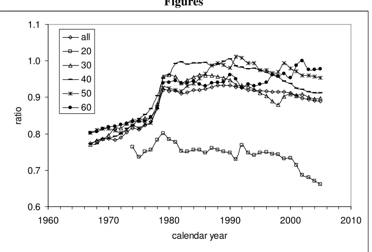
In the youngest age group between 16 (15 before 1987) and 24 years of age, only

65% to 80% reported some income, as presented in Figure 1. Corresponding curve has a

peak in 1979. Since then, the portion of people with income in this age group has been

decreasing. This effect, obviously, needs a thorough consideration and might be induced by

the appearance of some new actual sources of income not included in contemporary CPS

questionnaires. An increasing level of intra-family income redistribution is a potential

mechanism to consider.

Figure 1 demonstrates that the portion of people with income increases with age

before reaching its peak and then falls again. In 2005, the largest potion was measured in the

group between 55 and 64 years of age and reached 98%. This observation is consistent with

the fact that critical work experience, Tcr, in our model was moved in this age group (see

Section 1 for details). Between 1967 and 1977, the curves for all age groups except the

youngest one were converging, and after 1979 the scatter of the curves is almost constant.

An important observation is the step in all distributions (except the youngest one) between

introduction of new income definitions and significant changes to the CPS methodology. In

average, this step is around 10%. For example, the portion of population with income in the

working age population as a whole jumped from 83% in 1977 to 92% in 1979. One can

expect that further elaboration of income definition will result in 100% participation in

income distribution: there should be no persons without income.

For people of 44 years of age and above, the portion with income is more than 95%.

Therefore, in corresponding age groups, the difference between Gini coefficient associated

with people having income and that associated with the working age population as a whole

has to be the smallest among all age groups. These age groups provide the best opportunity

to test our model because almost everybody has some reported income.

Information on each and every individual income is not available. In this situation,

Gini coefficient can be estimated approximately. For example, if (Xi,Yi) are the values

obtained from the CPS, with the Xi indexed in increasing order (Xi-1 < Xi ), where Xi is the

cumulated proportion of the population variable, and Yi is the cumulated proportion of the

income variable, then the Lorenz curve can be approximated on each interval as a straight

line between consecutive points and

G = 1- (Xi-Xi-1)(Yi-1 + Yi), i=1,…,n (5)

is the resulting approximation for G.

In addition, one can approximate the Lorenz curve between consecutive points

(Xi,Yi) using exponential function or power law (where it is appropriate) for the

interpolation of underlying PIDs, as proposed by Dragulesku and Yakovenko (2001). The

choice of appropriate function for the PID interpolation reveals an important problem of the

CPS - the usage of the same income bins during relatively long periods of time. The growth

rate of nominal GDP in the U.S. has been high - more people obtained larger incomes above

the predefined upper income limit in CPS questionnaire and found themselves in the group "

$MAX and over". So, the coverage of population below and above the Pareto threshold,

which has been also proportionally growing, has been changing significantly. This variation

corresponding bias in the estimations of Gini coefficient. Also, under-coverage of the

highest incomes is a potential source of on-going discussion about increasing income

inequality in the U.S.. The absence of good quantitative estimates results in a wrong

interpretation of income inequality (Kitov, 2007b).

In the income range below the Pareto threshold, one can use quasi-exponential

distribution and estimate mean income in relevant bins. In the high-income zone, a power

low approximation is a natural choice for the PIDs. Theoretically, the cumulative

distribution function, CDF, for the Pareto distribution is defined by the following

relationship:

CDF(x) = 1 - (xm /x)k

for all x>xm,, where k is the Pareto index. Then, the probability density function, pdf, is

defined as

pdf(x) = kxmk/x k+1 (6)

Functional dependence of the probability density function on income allows an exact

calculation of total population in any income bin, total and average income in this bin, and

the input of the bin to corresponding Gini coefficient because the pdf defines the Lorenz

curve. Thus, if populations are counted in some predefined income bins, then relevant

Lorenz curve can be constructed for a given value of the Pareto index, k. We use (6) in the

following calculations of empirical Gini coefficients in the Pareto zone in all age groups. By

definition, the Pareto threshold evolves proportionally to nominal GDP per capita, and does

not depend on age.

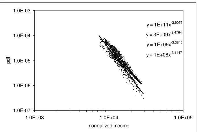
Index k, however, depends on age, as Figure 2 demonstrates. The evolution of the

Pareto law index (slope) with age is as follows: k=-1.91 for the age group between 25 and 34

years; k=-1.48 between 35 and 44; k=-1.38 between 45 and 54; k=-1.14 in the age group

between 55 and 64. It is clear that index k declines with age. Obviously, smaller index k

decrease in k deserves a special study because it should be inherently linked to some

age-dependent dynamic processes above the Pareto threshold.

Also, the declining k is a specific feature of the age-dependent PIDs, which should

be incorporated in our model. Kitov (2007a) found that k=-1.35 for the population of 15

years of age and over, i.e. within the range of its change with age. One can expect, however,

that the age-dependent and overall k might also undergo some changes over time. The latter

index may vary just because of changing age pyramid, i.e. changing input of various ages to

the net k. For the empirical estimates of Gini coefficients carried out below, the observed

variation in this index plays insignificant role because we use actual income distributions.

For the theoretical estimates in Section 3, Gini coefficient might be overestimated for the

youngest age group and underestimated in the oldest age group when one uses k=-1.35.

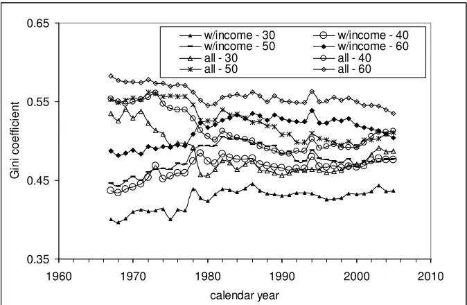
The U.S. Census Bureau (2006) presents two versions of PID – for total working age

population and for that with some reported income. We have calculated empirical G-values

in several (fixed) age groups between 1967 and 2005. Figure 3 displays the evolution of

Gini coefficient in all groups except in the youngest one. The latter group is characterized by

severe variations in methodology and definition of income. This makes it impossible to

distinguish actual and artificial features in the evolution of G. The curves associated with all

people aged in given ranges are marked “all”, and those including only people with reported

incomes – “w/income”. The major revision to income definition between 1977 and 1979,

which dramatically increased the portion of people with income, induced sharp decrease in

the curves named “all”, and opposite changes in the curves “w/income”. For obvious

reasons, the Gini coefficients for people with income are systematically lower than those for

the entire population. The curves in Figure 3 have to be predicted by our model.

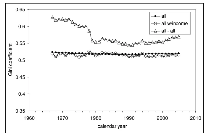
One important feature of the empirical Gini curves was also mentioned in (Kitov,

2007a). Before 1977, the portion of population without income was big enough to introduce

a significant bias in the estimates of Gini coefficient. It was overestimated for the entire

population and was underestimated for the population with income. Same effect is observed

for the age-dependent Gini. Before 1977, one can observe large changes over time. After

1977, all curves are approximately horizontal, with only a slight decline. Hence, one can

The accuracy of theoretical estimates of Gini coefficient is related to the quality of

PIDs' prediction. Figure 3 indicates that the Gini coefficients for the age groups over 34

years vary in a narrow range. This observation presumes that underlying PIDs are very

similar.

Kitov (2007a) demonstrated that the PIDs for the entire working age population

(with income) for the years between 1967 and 2005 collapse practically to one curve when

normalized to populations and nominal GDI (instead of GDP). Real GDP drives two key

parameters in our model: critical work experience, Tcr, and the size of earning tools, Λ(t).

However, when GDI is not equal GDP (as assumed in the model) one should use the former

variable for the normalization of the PIDs. GPI/GDP ratio has been varying through time

since the start of the CPS. Introduction of new sources of income in the CPS questionnaires

results in some increase in the GPI in addition to true changes in true GPI. The portion of

GPI (BEA, 2008) in the U.S. GDP increased from 0.76 in 1951 to 0.86 in 2001. A drop in

the portion was observed between 2001 and 2005 – from 0.86 to 0.82.

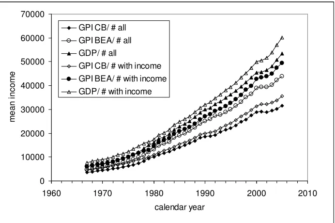
Figure 4 presents the evolution of various measures of mean income (i.e. GPI per

capita) using: GDP; GPI reported by the BEA; and GPI reported by the Census Bureau, as

estimated in annual CPS. Two population estimates are used for calculations of these mean

values – total working age population (all) and people reporting income (with income).

According to current income definitions, the GPI reported by the BEA is larger than that

estimated by the CB because the former includes additional sources of income. By mistake,

the BEA’s GPI was used in the modeling of the overall PID (Kitov, 2007a).

In the case of age-dependent PIDs, one should separately estimate total personal

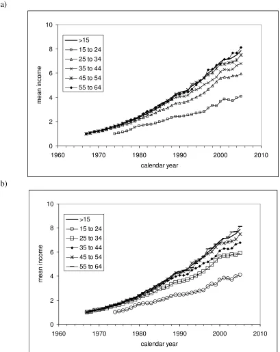
income in each age group. Similar to Figure 4, in Figure 5 we present the evolution of mean

personal income in various age groups. There are two cases shown: for all people of given

age (including those with no income) and for people who reported income. (By definition,

mean personal income is the ratio of total personal income and relevant population.) One

can observe dramatic differences between the youngest people and those in the groups with

the largest mean income. The curves obtained from the estimates provided by the Census

Before normalizing the age-dependent PIDs to total income and population one

needs to reduce them to the same units. Originally, the PIDs are obtained in income bins of

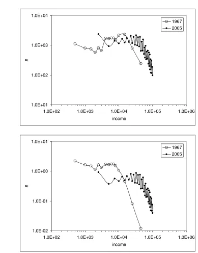
different width. For example, Figure 6a displays the PIDs for the age group between 35 and

44 years in 1967 and 2005. Income bins are not uniform in 1967 creating local troughs and

peaks. In 2005, income bins are uniform between $0 and $100,000. Obviously, the number

of people in a given bin depends on its width and position in the distribution. A reasonable

way to reduce these inhomogeneous distributions to the same units is to divide the number

of people in a given bin by its width. This mathematical operation defines population

density, i.e. the number of people per $1 at given income level. For the sake of simplicity,

we assign the obtained readings of density to the centers of relevant bins. Figure 6b depicts

the PIDs (shown in Figure 6a) normalized to the width of relevant income bins. The troughs

and peaks are essentially smoothed in the density curves. It is likely that true population

density distribution can be represented by an exponent undergoing a smooth transformation

into a power law function near the Pareto threshold (Yakovenko, 2003).

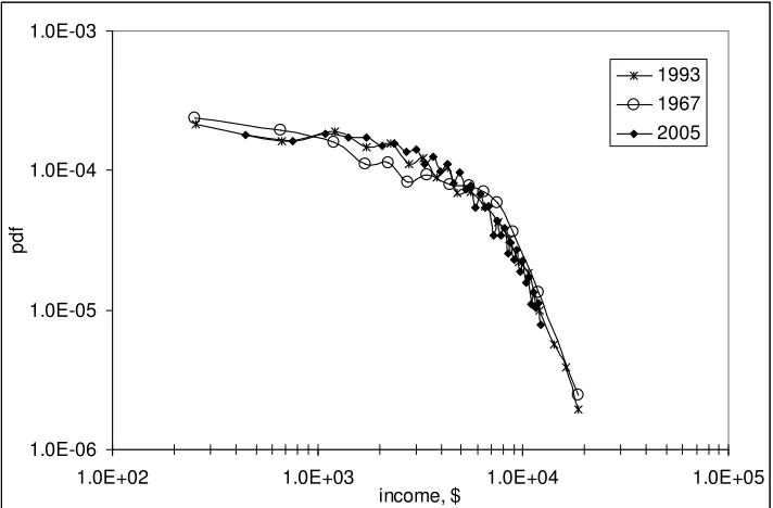
Finally, we have population density curves, which are defined in the same units. To

reduce them to one scale we normalize them to total population in relevant age intervals and

to the increase in total income over years, as presented in Figure 5. We expect that the

normalized curves should collapse to one within the bounds of uncertainty related to

measurement errors. Figure 7 shows the normalized PIDs in various age groups for people

for years 1967, 1993, and 2005. There is no significant difference between the curves except

in the age group between 16 and 24 years of age. We exclude the latter age group from the

modeling due to very high uncertainty in income measurements. The overall PIDs are also

shown as a corrigendum to those in (Kitov, 2007a).

This is the similarity between the normalized PIDs that results in practically constant

Gini coefficients in given age groups between 1967 and 2005. On the other hand, this

similarity supports our basic assumption that relative distribution of personal income has not

been changing over time not only overall, as shown by Kitov (2007a), but also for any given

age. One can conclude that there exist internal (economic, social, etc.) forces, which return

U.S. economy. This is an observation, not an assumption. To obtain theoretical estimates of

age-deponent Gini coefficients we start with the modeling of corresponding PIDs.

3. Comparison of observed and predicted Gini coefficients

Following our analysis of the observed age-dependent PIDs in Section 2 we have predicted

PIDs in the same age groups. The model is characterized by a resolution of 1 year of age and

1 year in calendar time. Therefore, we aggregated all personal incomes in the age groups

predefined by the CPS. The start year of the model is 1967 with the following defining

parameters: α0=0.071; Tcr(1967)=32.0 years; MBPB(1967)=0.43. Index k is taken for given age

group from the empirical estimates in Section 2. Other parameters are the same as in (Kitov,

2007a) and described in Section 2. The age distribution of population was obtained from the

Census Bureau (2007). This distribution is prone to revisions, however. For selected age

groups, such revisions may reach several percentage points. This might result in slight

deviations in the predicted Gini coefficients.

Figure 8 displays predicted and observed PIDs for the age groups between 24 and 35

years of age, between 45 and 54 years of age, and for the whole population over 15 years of

age. For the narrow age groups, the PIDs measured in 1993 were chosen, and for the whole

working age population the year of 2005 was modeled. Corresponding indices are those

estimated empirically and are as follows: k=-1.91; k=-1.38, and k=-1.35. These values fit the

roll-off in relevant PIDs’ above the Pareto threshold. In the low-income zone, the best fit is

observed for the whole population. This is likely the result of better resolution in the entire

population curve al lower incomes in 2005. In 1993, the resolution at low incomes was poor.

This was one of the reasons for new questionnaire and methodology introduced in 1994. The

number of income bins underwent a dramatic increase from 23 (including the open-end one

for the highest incomes) to 42. All in all, the observed and modeled PIDs demonstrate very

good similarity, which should be reflected in Gini coefficients.

The model predicts the evolution of each and every personal income. Therefore, it

allows the prediction of an exact Gini coefficient for a given set of defining parameters

because the construction of the Lorenz curve is possible. The empirical Gini coefficients

These empirical coefficients provide only some estimates of the range, within which true

age-dependent Gini coefficients are likely to reside.

Figure 9 presents the evolution of the observed and predicted Gini coefficient in four

age groups and for the whole population over 16 years of age. For the sake of simplicity, we

predicted Gini using the same index k=-1.35. In the age group between 25 and 34 years of

age, the predicted curve is close to that obtained for the entire population in this group.

Because actual index is k=-1.91, there is a slight overestimation of the predicted coefficient,

but it still resides between the empirical curves. Since 1994, the predicted curve has been

deviating from the curve for the whole population and approaching that for population with

income. This might be an effect of a higher resolution related to the introduction of new

income bins.

In the age group between 35 and 44 years of age, the empirical curves are closer to

each other. The predicted curve stays between them, but much close to the curve for

population with income. In the age group between 45 and 54, where theoretical index k is

close to actual one, the predicted curve reproduces the decline in both empirical curves

observed after 1983 and lays much close to the empirical curve for population with income.

This is likely that the true Gini coefficient in this age group is consistent with the predicted

one. In the age group between 55 and 64, the predicted curve is also close to that for the

working age population, but still between the empirical curves. As expected, the level of

income inequality in this age group is larger than in any other age group.

It is worth noting that the gap between the empirical Gini curves is between 0.02 and

0.03. The gap between the predicted and empirical curves is usually less than 0.01. This is

less than the uncertainty of the estimation of Gini coefficient as related to the discrete

representation of the observed PIDs.

In all age groups, the level of personal income inequality, as expressed by Gini

coefficient, has been decreasing (with small local peaks) since 1967. This empirical and

theoretical observation is especially important for the age groups above 45 years, where the

portion of population with income is close to 100%.

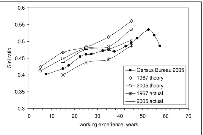
The predicted and measured curves demonstrate that the true Gini coefficient is age

this study for 1967 and 2005, two theoretical curves predicted by our model, and a curve

reported by the Census Bureau. Due low resolution large measurement errors in the

youngest and oldest age groups we limit our study to the age between 25 and 65. In this

range, all curves are very close. However, the CB’s curve goes beyond the limits and

demonstrates that there is a turning point at the age between 65 and 70. Our model supports

this observation and the average income for people above the critical age, Tcr, rolls-off

exponentially with age. This fast decay is also reflected in a severe drop in the number of

people with income above the Pareto threshold and corresponding decrease in Gini

coefficient.

Conclusion

This study was primarily carried out for validation of the microeconomic model defining the

evolution of personal incomes in the U.S. Our previous paper (Kitov, 2007a) revealed some

problems with income definition, which did not allow a comprehensive description of the

overall PID. The most important problem was that a large portion of population did not

report any income. Another problem is a poor resolution of PIDs before 1977.

In the model, everyone is assigned a non-zero income. This discrepancy results in a

significant deviation between observed and predicted Gini coefficients. The age-dependent

PIDs allow overcoming this discrepancy because the portion of population without income

is very low (~2%) for ages over 45 years. Therefore, one could assume a more precise

prediction of Gini coefficient in these age groups. This paper confirms this assumption: the

evolution of Gini coefficient for the years with a good PID resolution was accurately

(<0.005) predicted.

I would not like to repeat here all conclusions from (Kitov, 2007a). They are all right

and validated in this paper. In order to unbiased estimates of (also age-dependent) Gini

coefficient, one needs precise definition of personal income, i.e. the definition under which

GPI equals GDP, higher and uniform resolution, and accurate measurements.

As expected, the gap between the Gini coefficient associated with the entire working

population in a given age interval and that associated with people reporting income converge

somewhere between these two estimates. In the group between 45 and 54 years of age, this

portion is approximately 3% and the gap is less than 0.02.

As the overall PIDs, the empirical age-dependent (density) PIDs collapse to

practically one curve when normalized to cumulative growth in personal income and total

population for the period between 1967 and 2005.

In all age groups, the model predicts slightly decreasing Gini coefficients between

1967 and 2005. The overall G is approximately constant, however. Minor changes in the

overall G are related to economic growth and changes in the age structure of American

population.

The Pareto law index, k, undergoes significant changes over age: increases from the

youngest age to approximately 67 years of age, and then drops. Such an evolution could be

expected but its actual behavior deserves a deeper study.

The age-dependent PIDs demonstrate a fixed hierarchy during a very long period

between 1967 and 2005. It is unlikely that this hierarchy will be destroyed in near future.

The shape and the evolution of the measured PIDs are well predicted for the whole period.

This allows exact prediction of Gini coefficient and other measures of inequality, which are

defined by personal income distribution. Therefore, these measures of income inequality are

References

Bureau of Economic Analysis, (2008). National Economic Accounts, Tables, Retrieved on March 30, 2008. http://bea.gov/bea/dn/nipaweb/Select Table.asp?Selected=Y

Dragulesky, A., and Yakovenko, V., (2001). Exponential and power-law probability distributions of wealth and income in the United Kingdom and the United States. Physica A: Statistical Mechanics and its Applications, 299, 1-2 , 213-221.

Kitov, I., (2005a). A model for microeconomic and macroeconomic development, Working Papers 05, ECINEQ, Society for the Study of Economic Inequality. www.ecineq.org/milano/WP/ECINEQ2005-05.pdf.

Kitov, I., (2005b). Modeling the overall personal income distribution in the U.S. from 1994 to 2002, Working Papers 07, ECINEQ, Society for the Study of Economic Inequality. www.ecineq.org/milano/WP/ECINEQ2005-07.pdf.

Kitov, I., (2005c).Evolution of the personal income distribution in the U.S.: High incomes, Working Papers 02, ECINEQ, Society for the Study of Economic Inequality. www.ecineq.org/milano/WP/ECINEQ2005-02.pdf.

Kitov, I., (2006). Modeling the age-dependent personal income distribution in the U.S., Working Papers 17, ECINEQ, Society for the Study of Economic Inequality. www.ecineq.org/milano/WP/ECINEQ2006-17.pdf.

Kitov, I., (2007a). Modeling the evolution of Gini coefficient for personal incomes in the U.S. between 1947 and 2005, Working Papers 67, ECINEQ, Society for the Study of Economic Inequality. www.ecineq.org/milano/WP/ECINEQ2007-67.pdf.

Kitov, I., (2007b). Comparison of personal income inequality estimates based on data from the IRS and Census Bureau, MPRA Paper 5372, University Library of Munich, Germany, http://ideas.repec.org/p/pra/mprapa/5372.html.

Neal, D. and Rosen, S., (2000). Theories of the distribution of earnings. In: Handbook of Income Distribution, (Eds.) Atkinson, A. and Bourguinon, F., 379-427, Elsevier 2000.

Rodionov, V.N., Tsvetkov, V.M., and Sizov, I.A., (1982). Principles of Geomechanics. Nedra, Moscow, p.272. (in Russian)

U.S. Census Bureau, (2000). The Changing Shape of the Nation's Income Distribution. Retrieved February 26, 2007 from http://www.census.gov/prod/2000pubs/p60-204.pdf.

U.S. Census Bureau, (2002). Technical Paper 63RV: Current Population Survey - Design and Methodology, issued March 2002. Retrieved February 26, 2007 from http://www.census.gov/prod/2002pubs/tp63rv.pdf.

U.S. Census Bureau, (2005). Changes in Methodology for the March Current Population

Survey, Retrieved February 26, 2007 from

http://www.census.gov/hhes/www/income/histinc/hstchg.html.

U.S. Census Bureau, (2007). Population Estimates. Retrieved March 14, 2007 from http://www.census.gov/popest/archives/

.

Figures

0.6 0.7 0.8 0.9 1.0 1.1

1960 1970 1980 1990 2000 2010

calendar year

ra

ti

o

all 20 30 40 50 60

y = 1E+08x-3.1447 y = 1E+09x-3.3845 y = 3E+09x-3.4764 y = 1E+11x-3.9075

1.0E-07 1.0E-06 1.0E-05 1.0E-04 1.0E-03

1.0E+03 1.0E+04 1.0E+05

normalized income

p

d

f

0.35 0.45 0.55 0.65

1960 1970 1980 1990 2000 2010

calendar year

G

in

i

c

o

e

ff

ic

ie

n

t

w/income - 30 w/income - 40

w/income - 50 w/income - 60

all - 30 all - 40

all - 50 all - 60

0 10000 20000 30000 40000 50000 60000 70000

1960 1970 1980 1990 2000 2010

calendar year

m

e

a

n

i

n

c

o

m

e

GPI CB/ # all GPI BEA/ # all GDP/ # all

GPI CB/ # with income GPI BEA/ # with income GDP/ # with income

a) 0 2 4 6 8 10

1960 1970 1980 1990 2000 2010

calendar year m e a n i n c o m e >15 15 to 24 25 to 34 35 to 44 45 to 54 55 to 64

b) 0 2 4 6 8 10

1960 1970 1980 1990 2000 2010

calendar year m e a n i n c o m e >15 15 to 24 25 to 34 35 to 44 45 to 54 55 to 64

a)

1.0E+01 1.0E+02 1.0E+03 1.0E+04

1.0E+02 1.0E+03 1.0E+04 1.0E+05 1.0E+06

income

#

1967 2005

b)

1.0E-02 1.0E-01 1.0E+00 1.0E+01

1.0E+02 1.0E+03 1.0E+04 1.0E+05 1.0E+06

income

#

1967 2005

a) 16 to 24

1.0E-07 1.0E-06 1.0E-05 1.0E-04 1.0E-03

1.0E+02 1.0E+03 1.0E+04 1.0E+05

income, $

p

d

f

1974 2005

b) 25 to 34

1.0E-07 1.0E-06 1.0E-05 1.0E-04 1.0E-03

1.0E+02 1.0E+03 1.0E+04 1.0E+05

income, $

p

d

f

c) 45 to 54

1.0E-06 1.0E-05 1.0E-04 1.0E-03

1.0E+02 1.0E+03 1.0E+04 1.0E+05

income, $

p

d

f

1967 1993 2005

d) 55 to 64

1.0E-06 1.0E-05 1.0E-04 1.0E-03

1.0E+02 1.0E+03 1.0E+04 1.0E+05

income, $

p

d

f

e) 16 years of age and over

1.0E-06 1.0E-05 1.0E-04 1.0E-03

1.0E+02 1.0E+03 1.0E+04 1.0E+05

income, $

p

d

f

1993 1967 2005

a) 25 to 34 years of age

1.0E-07 1.0E-06 1.0E-05 1.0E-04 1.0E-03

1.0E+02 1.0E+03 1.0E+04 1.0E+05

income, $

p

d

f

1993 measured 1993 theoretical

b) from 45 to 54 years of age

1.0E-06 1.0E-05 1.0E-04 1.0E-03

1.0E+02 1.0E+03 1.0E+04 1.0E+05

income, $

p

d

f

c) over 16 years of age

1.0E-06 1.0E-05 1.0E-04 1.0E-03

1.0E+02 1.0E+03 1.0E+04 1.0E+05

income, $

p

d

f

2005 measured 2005 theoretical

Figure 8. Comparison of measured and predicted PIDs in some age groups. High incomes are describes by a power (Pareto) law with index k=-1.91; k=-1.38; and

a)

0.35 0.4 0.45 0.5 0.55

1960 1970 1980 1990 2000 2010

calendar year

G

in

i

ra

ti

o

25-34 income - 30 all - 30

b)

0.4 0.45 0.5 0.55 0.6

1960 1970 1980 1990 2000 2010

calendar year

G

in

i

ra

ti

o

35-44 income - 40 all - 40

c)

0.4 0.45 0.5 0.55 0.6

1960 1970 1980 1990 2000 2010

calendar year

G

in

i r

a

ti

o

45-54 w/income - 50 all - 50

d)

0.45 0.5 0.55 0.6

1960 1970 1980 1990 2000 2010

calendar year

G

in

i

ra

ti

o

e)

0.35 0.4 0.45 0.5 0.55 0.6 0.65

1960 1970 1980 1990 2000 2010

calendar year

G

In

i

c

o

e

ff

ic

ie

n

t

all

all w/income all - all

0.3 0.35 0.4 0.45 0.5 0.55 0.6

0 10 20 30 40 50 60 70

working experience, years

G

in

i

ra

ti

o

Census Bureau 2005 1967 theory 2005 theory 1967 actual 2005 actual