Advances in classification of EEG signals via evolving fuzzy classifiers and dependant multiple HMMs

Advances in Classification of EEG Signals via

Evolving Fuzzy Classifiers and Dependant Multiple

HMMs

C. Xydeas, P. Angelov, C. Shih-Yang, M. Reoullas

Digital Signal Processing Group Department of Communication Systems

Infolab21, Lancaster University Lancaster, LA1 4WA, UK

Phone: +44-1524-510310 Fax: +44-1524-592713

Abstract: Two novel approaches to the problem of brain signals (EEG) classification

are introduced in the paper. The first method is based on a modular probabilistic network

architecture that employs Multiple Dependant Hidden Markov Models (DM-HMM-D) on the

input features (channels). The second method, eClass, is based on an on-line evolvable fuzzy

rule base of EEG signal prototypes that represent each class and take into consideration the

spatial proximity between input signals. Both approaches use supervised learning but differ

in their mode of operation. eClass is designed recursively, on-line, and has an evolvable

structure, while DM-HMM-D is trained off-line, in a block-based mode, and has a fixed

architecture. Both methods have been extensively tested on real EEG data that is recorded

during several experimental sessions involving a single female subject who is exposed to mild

pain induced by a laser beam. Experimental results illustrate the viability of the proposed

approaches and their potential in solving similar classification problems. © Elsevier 2006

Keywords: EEG, HMM networks, on-line evolving clustering, evolving fuzzy rule-based

1. INTRODUCTION

1.1 EEG in the context of brain-computer interaction

The human brain is the most complex information processing system known to science. It is this

complexity that has attracted the interest of many scientists over the past years in studying the

physiological activity of the brain. Human brain activity can be recorded in the form of

electroencephalogram (EEG) signals. These provide an important source of information which can be

useful in the study of underlying brain processes as well as in a variety of medical applications i.e. the

use of EEG signals for psychiatric/physiological diagnosis as well as for evaluation of sensory

experiences [1]. A particularly interesting aspect of EEG signal analysis is that related to pain

experiences. From a medical point of view, the pain sensation is important either because of its mere,

unpleasant presence or because it inhibits physiological functions or because it can be related to

certain pathological conditions. These are a major source of disability, poor health status and

mortality. The ability to analyze EEG signals and to interpret accurately different aspects of the pain

sensation can be a major advance in pain research and clinical pain management. Previous work has

shown that analysis of pain can be possible with the help of powerful techniques based on coherence

analysis and topographic mapping. Thus EEG coherence analysis provides a measure of functional

correlations between EEG signals [1–5] whereas functional imaging techniques have identified the

matrix of brain structures that are responsible for the elaboration of pain experience. The precise

division of function within this matrix is unclear.

The general thrust of the work presented in this paper is to develop practically feasible

“intelligent” computer based systems for processing EEG brain activity information. Furthermore, the

specific EEG signal analysis issue addressed here is that of pain detection, a capability that can find

extensive use in the medical area, for example in real-time pain monitoring of patients under

anesthesia, or in the safety/defense field, for example in real–time pain detection monitoring of

two and substantially different EEG signal classification methodologies (i.e. DM-HHM-D and

e-Class) which have been developed and employed within the context of real-time pain detection. These

classification techniques employ supervised learning in their classification system design, with the

DM-HHM-D technique relying on the a priori (off-line) provision of representative training data and

has a fixed system architecture whereas the e-Class method is capable of formulating the

classification system architecture and associated fuzzy rules/parameters on-line and “from scratch”

while processing and classifying given input EEG signals. Furthermore, given the fuzzy rules

designed from previous data, e-Class is capable of updating and generalizing its set of rules by further

recursive on-line training using new data.

1.2 HMM and DM-HMM-D

The theory of Hidden Markov Models (HMMs) [7]-[9] is a rigorous probabilistic classification

framework that has been successfully applied to several applications domains [10]-[12]. Furthermore,

their natural capability of dealing with time varying patterns of arbitrary lengths is attractive due to

the expected variability in the time lengths of dynamic signal patterns. In most real-time classification

applications (i.e. pain/no pain EEG signals classification) several different signals or features are

observed (i.e. 64 EEG channels from the brain cap) in order to increase recognition/classification

performance.

When dealing with multiple features having discrete observation densities, two HMM system

design approaches can be used [8,10]: The first, HMM-VQ, employs Vector Quantization (VQ) to

account for any dependencies that may exist between the input features whereas the second approach,

IM-HMM-D, is based on the “separation” of input features and the assumption of no significant

dependency between input features. The main drawback of the VQ based approach is that

classification system performance can be reduced significantly if an inappropriate VQ method (in

terms of quantization accuracy) is chosen [11]. Furthermore, due to system complexity limitations,

possible, which in turn leads to a feature selection search process. In addition when a new feature is

added or an old feature is removed, codebooks must be re-designed and HMM networks

retrained/redefined.

The second method [10][13] is based on a “multi-HMM-D” system formulation (hereafter

referred to as IM-HMM-D) that employs in parallel separate HMM networks per input feature and

combines their outputs in order to formulate an overall classification result. Furthermore a novel

multiple HMM-D system architecture is presented in this paper that computes dynamically with time

“weights” associated to the observed values of different features and employs them in the formulation

of the overall classification result, according to the varying-with-time importance of the input

features. This proposed classification structure, named as DM-HMM-D, aims to fully and efficiently

exploit any inter-dependencies that may exist between input features.

1.3 Evolving Classifier (e-Class)

An important aspect in the analysis of EEG signals is the relevance of the classification system results

and the system’s generalization capability. Very often [6] EEG data are extracted from a small

number of subjects or even a single subject, as in the case of the present study. Experimental

configuration may vary, including the mental and physical condition of the subject (expectation,

anxiety etc.). As a result, classifiers which are trained in a “batch” mode with a fixed set of training

data may become irrelevant or imprecise when applied to scenarios characterized by new operating

conditions. One possible solution to this problem is to design classifiers that can be recursively

updated, or self-organizing classifiers.

Recently proposed schemes concerning evolving un-supervised clustering [26] and evolving Self

Organizing Maps (SOM) [15] can be extended to the case of supervised learning (labeled outputs).

These self-organizing classifiers are also called evolving, because they develop their structure of

prototypical samples starting “from scratch“, using the input EEG signals and their accumulated

generic and can be applied to other classification problems, such as on-line classification of difficult

targets [25].

Paper Organization

The remaining of this paper is organized as follows. Section 2 gives an insight on the procedure used

for EEG data collection and includes some technical information on data acquisition and data

preprocessing techniques. Section 3 discusses HMM systems in general and the novel DM-HMM-D

scheme in particular, emphasizing its main characteristics and resulting advantages as compared to

conventional HMM-D. Section 4 introduces a novel on-line recursive approach to the classification of

EEG signals, called eClass, where the structure of the classifier evolves to take into account the

changing characteristics of the processed EEG signals. This classification method is generic and is

ideally suited for use in on-line type of applications where the architecture of the classification system

is not predetermined [25]. Section 5 gives an account and analysis of the experimental results

obtained from both methods operating on the same real data. Finally, section 6 concludes this paper

with a summary of the comparative investigations presented in previous sections and identifies future

work aimed at achieving further improvements in EEG pain classification results.

2. EXPERIMENTAL CONFIGURATION

Repeated heat stimuli in the form of laser pulses were delivered in a controlled manner by laser

cannon (CO2 laser) to the right forearm of the subject. The duration of each pulse is set to 150ms, and

each such stimulus is repeated at regular intervals of 10s (epochs). Each EEG continuous recording

included 61 stimuli. Note that EEG (channel) signal responses to the first stimulus were routinely

discarded, as they were considerably higher in amplitude, due to an element of “surprise” that is often

exhibited by the subject and associated artefacts in the EEGs. Thus, 60 stimuli were taken into

subject. These data files were recorded on three different days (i.e. 08.06.00, 15.06.00 and 02.08.00)

with three EEG recording sessions taken on each of the above three days.

More specifically, this EEG data collection experimental procedure can be described as follows:

1) The subject was seated comfortably in a chair, placed his/her arm on a table and the laser

cannon was positioned at a fixed distance from the subject’s hand.

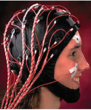
2) Electrodes were placed around the scalp, the eyes (to test whether the subject blinks) and on

each ear (which are used as “ground” for EEG), see Figure 2.1.

Figure 2.1 here

3)A computer is placed in front of the subject, showing a table with the pain intensity scale. The

subject was asked to rate the pain intensity of each stimulus using a scale from 0 to 10, where 0

represents no sensation and 10 represents unbearable pain. In these experiments the rating of 4

(“just painful”) was used as a pain threshold (i.e. 1–3: non–painful and 4–10: painful). Subjective

pain ratings were also recorded so that they could be used as “target” classification data during the

training and testing procedures of the proposed classification algorithms.

4) EEG readings taken from the electrodes were then stored automatically in a file using a control

program that also operated the laser cannon.

Thus recordings were made using a 64–electrode cap (see Figure 2.1) with 62 head electrodes while

two face electrodes (vEOG and hEOG) were used to monitor artifacts from eye movement. It must be

mentioned here that EEG artifacts associated with signal activity in electrodes vEOG and hEOG were

appropriately removed prior to the pain classification experiments.

Figure 2.2 here

EEG signals were band–pass filtered at 0.15–30Hz and sampled at a frequency of 500Hz, with a gain

of 500 (150 for the EOG channels). Following the above described acquisition process of Pain/No

corresponding to (a) “Pain” signal states, represented by 1s intervals starting from the time of the pain

stimulus, and (b) “No Pain” signal states represented by 1s intervals centred at 1s before the

application of each pain stimulus.

3. DM-HMM-D

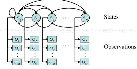
The general structure of a one-feature discrete observation HMM network is shown diagrammatically

in Figure 3.1.

Figure 3.1 here

There are N hidden states (nodes) {S1,S2,…,SN} in the model and M possible observations can be

generated by the model. At every time step one of the states, say Sj, is entered based on the state

transition probability {aij} that depends on the previous state Si. After each transition is made, an

observation, say the m-th observation om, is produced from Sj with corresponding observation

probabilities {bj(om)}, note that the initial state probabilities are defined as {πi}. A compact notation

λ={{aij},{bj(om)},{πi}} is set to indicate the complete model parameters. Therefore, the probability of

an given observation sequence O={o1,o2,…,oT} in the period of time T can be calculated by tracing the

paths Q={q1,q2,…,qT} (Viterbi paths) which offer the maximum likelihood probability P(O|λ).

Equation 3.1 shows the result of multiplying all the probabilities that the Viterbi path passes through.

Note that f(π,a) is a function of initial probabilities and state transition probabilities.

∏

∏

1 ) ( ) ( 2 ) ( ) ( 1 2 1 ) ( ) , ( ) ( ) ( ) ( ) ( ) ( ) | ( ) ( ) ( ) ( 1 -) ( 1 1 1 2 1 1 1 T k k q T k k q q q q q T q q q q q q q o b a f o b a o b o b a o b a o b O P k k k k T T T = = = = = = ₋ π π π λ _L (3.1)

A novel multiple HMMs system architecture (named DM-HMM-D, Figure 3.2) is introduced that

computes the weights attached to different sequences of observations prior to the operation of HMM

models. Figure 3.2 (a) shows the conventional IM-HMM-D model framework and the final

probability likelihood in the IM-HMM-D is computed as shown in Equation 3.2 which assumes that

c≠i are independent.

Figure 3.2 here

In this case C features {o(k)(1),o(k)(2),…o(k)(C)} are available, at a given time k, the system employs C

HMM parameter sets {λ1,λ2,…, λC} and the total likelihood probability P(O|λ) is given as:

∏

1

) | ) ( ( ) |

( C

i i

i O P O

P

=

= λ

λ (3.2)

This conditional independence is stated as

) | ( = ) , |

( () ()

i i i

i _{λ Y PO λ}

O

P (3.3(a))

where O(i)_={o1(i)_,…,oT(i)_{} is the observation sequence of the i-th feature and}

Y={O(1)_,O(2)_,…,O(c)_,…,O(C)_{}, c≠i are the observation sequences of the remaining features.}

In Figure 3.2 (b), different sequences of observations are considered to be “linked” in a vertical

manner by assuming that a weighting function is introduced to each model. The output probability of

the i-th model is rewritten as _P(_O()|ˆ) _w(_O) i i

i _λ , where

i

λˆ is the new HMM parameter set for the i-th feature.

Equation (3.2) can be rewritten as:

∏

1

)

( _|ˆ_{) ( ))}

( ( ) ˆ |

( C

i

i i

i _{w O}

O P O

P

= =

′ λ

λ _(3.3(b))

where wi(O) is designed to be the conditional probability of O(i) _{given Y, i.e. the probability of the}

observation sequence of the i-th feature given the observation sequences of the remaining features.

) | ( = )

(_{O p O}() _Y

w i

i (3.3(c))

The system shown in Figure 3.2(b) now takes the form shown in Figure 3.2(c) that can be also

depicted as in Figure 3.2 (d). This new Multi HMM model structure is named as DM-HMM-D, to

distinguish it from the conventional IM-HMM-D scheme. Since the weight function wi(O) and the

conventional HMM structure are now effectively combined, the HMM training and testing procedures

must be adjusted appropriately.

Considering Equations (3.3(b)), (3.3(c)) and (3.2), the conditional probability ₍ ()_|ˆ)′

i i _λ

O

p can be rewritten

∏

∏

∏

1 = ) ( ( ) ) ( ) ( ) ( ) ( ) ( ) ( ) ( 1 = )

( ( )=1 ( )

) ( ) ( ) ( ) ( ) ( ) ( ) ( ) ( ) ( ) ( ) | ( ) ( ) , ( = ) | ( ) ( ) , ( = ) | ( ) ˆ | ( = )′ ˆ | ( ) ( ) ( T k k i k i k i q i i T k T k k i k i k i q i i i i i i i y o p o b a π f y o p o b a π f Y O P λ O P λ O P k k (3.4)

where the product terms represent the transitional probabilities of the new model, i.e.

)

|

(

)

(

=

)

′

(

() _{( )} ) ( ) ( ) ( ) ( ) ( ) ( ) ( k i k i k i j i k i

j

o

b

o

p

o

y

b

(3.5)

It can be seen that the conditional independent probability P(O(i)_{|Y) will only affect observation}

transition probability {bj(i)_(o(k)(i)_{)}. Therefore DM-HMM-D can be implemented by replacing}

{bj(i)_(o(k)(i)_{)} with the probability {bj}(i)_(o(k)(i)₎’_{} at each time step (k).}

{bj(i)_(o(k)(i)₎’_{} is calculated using Equation (3.5) with the help of a pre-defined (during the training}

procedure) “dependency” codebook that contains p(o(k)(i)_{|y(k)) estimates. In particular, p(o(k)}(i)_|y(k))

estimates are obtained using:

i z i V i U h O O h T i V i U h T O O h y p y o p o o o o o p y o p K k T k k k k K k T k k k k K k k K k T k k k k K k K k k T k k k k k k i k C k c k k k i k k i k k k k k ≠ , )) ( ), ( ( ) , ( / )) ( ), ( ( / ) , ( ) ( ) , ( })) , , , , , ({ | ( ) (

∑ ∑

∑ ∑

∑

∑ ∑

∑

∑

∑

1( )'1

) ( )' ( , 1( )'1

) ( )' ( , 1 1()'1

) ( )' ( ,

1()'1 1

) ( )' ( , ) ( ) ( ) ( ) ( ) ( ) ( ) ( ) ( ) 2 ( ) ( ) 1 ( ) ( ) ( ) ( ) ( ) ( ) ( = = = = = = = = = = ₌ = =

= _{L L}

(3.6)

where Uk,(k)’(i)={ok,(k)’(1)_,ok,(k)’(2)_{,…,ok,(k)’}(c)_{,…,ok,(k)’}(C)_{} and V(k)(i)={o(k)}(1)_,o(k)(2)_,…,o(k)(c) _,…,o(k)(C)_{} with}

c≠ i are calculated as the expected number of times in observing V(k)(i) for all Uk,(k)’(i) in K training

data sets, k={1,2,…,K}. The counting function h(a,b) is equal to one if and only if {a=b}, otherwise its

value is zero.

The model evaluation and estimation procedures used in DM-HMM-D are effectively those

developed for conventional HMM-D structures with the simple replacement of {bj(i)_(o(k)(i)_{)} with}

{bj(i)_(o(k)(i)_)p(o(k)(i)_|y(k))}.

3.1 Model Evaluation

sequence length T and state number N.

The forward algorithm incorporates the following steps:

• Initialization: N i y o p o b

i) _{i i}( ) ( | ), 1≤ ≤

( _{1 1 1}

1 π

α = (3.7)

• Induction: N j T k y o p o b a i

j _{j k k k}

N

i

ij k

k ( ) [ () ] ( ()1) ( ( )1| ( )1), 1≤( )≤ ,1≤ ≤

1 ) ( 1 ) (

∑

+ + + =

+ =

α

α

(3.8) • Termination:

∑

1 = ) ( = ) , | ( N i T i α λ Y O P (3.9)

where the forward variable α(k)(i) is defined as α(k)(i)=P(o1 o2… o(k) , q(k)=Si/,λ)p(o(i)_{/y(k)). This}

formulation of the forward probability calculation is based on a lattice structure and is efficient since

the calculation of the forward variableα(k)(i) involves only N previous values of α(k)-1(i) [4].

The backward part of the process is similar to the Forward procedure with,

• Initialization:

N

i

i

T

(

)

=

1

,

1

≤

≤

β

(3.10) • Induction: 1 ,..., 2 , 1 = ) ( ; ≤ ≤ 1 ), ( ] ) | ( ) ( [ = )

( ( )+1

1 = 1 + ) ( 1 + ) ( 1 + ) ( )

( i

∑

a b o po y β j i N k T T

β k N j k k k j ij k (3.11) • Termination:

∑∑

1 = =1

1 + ) ( 1 + ) ( 1 + ) ( 1 + ) ( ) (

(

)

(

)

(

|

)

(

)

=

)

,

|

(

N i N j k k k k j ij

k

i

a

b

o

p

o

y

β

j

α

λ

Y

O

P

(3.12)

where the backward variableβ(k)(i) is defined as β(k)(i)=P(o(k)+1.. oT+2… oT| q(k)=Si,, λ) p(o(i)_/y(k)).

3.2 Model Estimation

The probability of P(O|Y, λ) is maximized via an iterative estimation process. Thus HMM parameter

model, noted as

λ

=

{

A

,

B

,

π

}

and a re-estimated modelλ ={A,B,π}. The expectation step E

involves the calculation of Baum’s auxiliary functionQ(λ,λ)) whereas the M (modification) step is

the maximization overλ. Re-estimation of a parameter set using K training data streams involves:

∑

1 = ) ( ) ( ) ( 1 ) ( 1 ) , | ( ) ( ) ( = K k k k k k

i _{P O Y λ}

i β i α π (3.13)

∑ ∑

∑ ∑

1 1 -1 ) ( ) ( 1 1 -1 ) ( 1 ) ( 1 ) ( 1 ) ( 1 ) ( ) ( ) ( ) ( 1 ) ( ) | ( ) ( ) ( 1 K k T t k t k t k K k T t k t k t k t k t k j ij k t k ij _k k i i P j y o p o b a i P a = = = = + + + + = β α β α (3.14)

∑ ∑

∑

∑

1 1 -1 ) ( ) ( 1 1 -. . 1 ) ( ) ( ) ( ) ( 1 ) ( ) ( 1 )

( _K ()

k T t k t k t k K k T o t s t k t k t k j _k k k t i i P i i P b = = = = = = β α β α l l (3.15)

In DM-HMM-D parameter sets λˆi={π

(i)_,a(i)_,b(i)_{}, i=1,…,C, are determined during training while using}

{bj(i)_(ot(i)_)p(ot(i)_{|yt)} instead of {bj}(i)_(ot(i)_{)} [14,15]. Following training, and during testing (i.e. when}

using the derived system to perform classification of input signals) the required probability P(O(i)_|Y)

for each input testing data stream is obtained from a pre-designed dependency codebook.

4. E-CLASS

As mentioned earlier, the relevance of the results produced by an off-line classification technique will

be limited to the degree of representativeness of the training data. The applicability of such an off-line

trained classifier to new data sets is limited and therefore, the design of incrementally evolvable

classifiers is an attractive alternative. Evolvable fuzzy-rule-bases have been recently developed and

successfully applied to clustering [26], time-series prediction [14,15], and neuro-fuzzy systems [24].

In this paper this concept [19] is extended to the on-line signal classification. The resulting novel

approach called eClass is based on an evolvable rule base, which is composed of fuzzy rules of the

Rulej_:

IF (EEG₁is EEG₁j*) AND …AND (EEG_n is EEG_nj*) THEN (Class is Pain/No Pain) (4.1)

where EEG_i denotes the electroencephalogram signal produced by the ith _{channel, i=1,2,…,n; in this}

particular application n=2, i.e. only the two most informative channels are employed (see

diagram representing the importance of all 64 channels in Figure 5.2). These channels have

been identified according to the wi(O) weight values of input features (indicating the relative

importance of corresponding channels) as estimated by the system described in section 3;

EEG_ij*denotes the jth prototypical EEG signal of the ith input (channel), i=1,2,…n; j=1,2,…,

Rk rules, k=1,2,… ,m

R is the number of fuzzy rules;

m is the number of classes (in this particular application m=2, namely: “Pain” and “No Pain”)

Class is the output of the classifier (in this particular application it is a binary variable with

values Pain/No Pain.

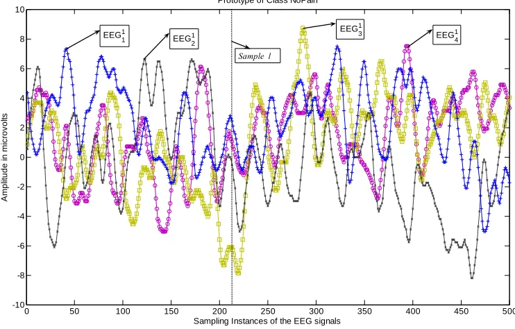
This overall rule base comprises of m sets of fuzzy rules – one per class, see Figure 4.1 where two sets

of prototypical EEG signals are depicted – one for the class “Pain” (Figure 4.1 (a)) and another for the

class “No Pain” (Figure 4.2 (b)).

Figure 4.1 (a) and (b) here.

The fuzzy rule base is designed in on-line mode via supervised learning starting “from scratch”. It

selects the first measured EEG signal as a prototype. Then, starting from the next measured EEG

signal, an accumulated proximity measure (called potential, [14, 19]) is calculated recursively and the

rule-base is incrementally updated. The potential, P is inversely proportional to the sum of Euclidean

distances between a particular EEG signal and all other EEG signals. The value of the potential will

be higher for these EEG signals that are similar to a large number of other EEG signals. It should be

modeling [15,22] techniques, in eClass the potential is calculated with respect to the inputs (discrete

EEG signals) only. Class labels (classifier outputs) are not included in the calculation of P.

The overall classification is performed based on the so called ‘winners take all’ principle [27],

which corresponds to the MAX t-norm used to produce a defuzzification (note that the same is also

used in Mamdani type fuzzy models) [18].

( )

j R

j

k k

y

y

λ

1

max arg ;

=

=

= _(4.2a)

∑

=

= R

j

j jy

y

1

λ

_(4.2b)

where yk represents the kth _{class, k=1,2,…m}

∑

=

= _R

i i j j

1

τ

τ

λ

_{is the normalized firing level of the j}th _{rule, j=1,2,…R.}

(

)

∑ ∑

=

= =

− − n

i L

l

l j l

i x

x

j

e

1 1

2 *

α

τ

is the firing rule of the jth fuzzy rule; j=1,2,…,R;

l j

x

is the jth_{sampled EEG signal;}

*

j

x

is the jth _{prototypical EEG signal based on which the j}th _{fuzzy rule antecedent is formed;}

α=4/r 2 _{is a positive constant which defines the spread of the membership function of the}

fuzzy sets which are of Gaussian type;

r is the radius that defines the zone of influence of the fuzzy rules;

L denotes the length of the discrete EEG signal.

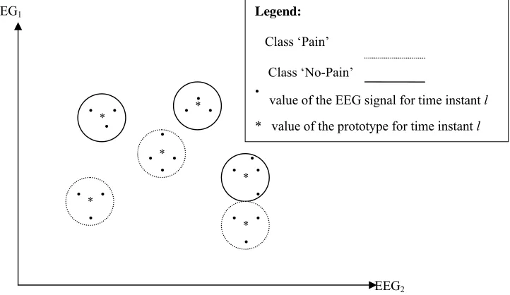
In Figure 4.2 a snap-shot, at given time instant k, of a 2-feature space is presented and two classes

(Pain and No Pain) are shown with different types of lines. It is important to mention that the

classification of EEG signals is performed based on similarity using the whole length of the EEG

Figure 4.2 here

The input data space in eClass is clustered on a per class basis. For each class the algorithm

forms a partial rule-base, which consists of Rk rules (k=1,2,… ,m). These class-related partial

rule-bases are then combined to form the overall rule-base R of the eClass process. In this way, the total

number of fuzzy rules that form the evolvable classifier R is equal to the sum of fuzzy rules that form

the partial rule-sets associated with each class, see Figure 4.3:

R= R1+R2+…+Rm (4.3)

Figure 4.3 here

It should be mentioned that the system learning and the testing procedures are performed in on-line

mode. EEG signals are first presented to eClass for classification and then (given the ground

truth/label) the same EEG signals are used to update or upgrade the partial rule-base, Rk of the (kth₎

class.

In eClass training, EEG signals are collected continuously. Some signals reinforce and confirm

the information contained in the classifier. Other input signals provide new information, which may

be important enough to form a new fuzzy rule or to modify an existing one. The value of the

information they contain can be measured by their potential, P. Two main potentials are calculated

recursively:

a) the potential of a EEG signal that is to be used as a new prototype; b) the potential of the existing prototype EEG signals.

Thus the potential of a new EEG signal to be a prototype of class j can be calculated recursively by

[26]:

[

]

) ( ) ( 2 )) ( 1 )( 1 (

1 )

(

k g k h k b k

k k

x P_k

+ − + −

−

= ; k=2,3,… (4.4)

where Pk(x(k))denotes the potential of the EEG signal x(k) calculated at the moment k;

∑∑

+

= =

=

1

1 1

2

)

)

(

(

)

(

n

j L

l l

j

k

x

k

b

;

∑ ∑ ∑

(

)

−

= +

= =

= 1

1 1

1

2

1

) ( )

( k

i n

j L

l l j i

x k

∑∑

+ = =

=

1 1 1

)

(

)

(

)

(

n j L l l j l

j

k

p

k

x

k

h

;

∑ ∑

−

= = = 1 1 1 ) ( ) ( k i L l l j l

j k x i

p

Parameters b(k) and h(k) are calculated from the current EEG signal x(k), while l

j

p (k) and

g(k) are recursively updated by

∑∑

+ = =

−

+

−

=

1 1 1 2

))

1

(

(

)

1

(

)

(

n j L l l j

k

x

k

g

k

g

;

p

(

k

)

=

p

(

k

−

1

)

+

x

l

(

k

−

1

)

j l

j l

j

A new input EEG signal is influencing the potentials of the established prototypes ( *

j

x , j=1,2,…,R), because by definition potentials depend on the distance to all of the input signals,

including the new one. The potential of a prototype ( *

j

x ) at

the moment

k

can be calculated as

[26]:

(

)

∑∑∑

− = + = = − + = ₁ 1 1 1 1 2 * )) , ( ( 1 1 1 1 ) ( _k p n i L l i l j p j d k k x

P

; k=2,3,…

(4.5)

where

_P

(

_x*(_k)

)

j

is the potential of the at the moment

k

of the cluster, which is a prototype of

the

j

th

rule;

) , (j p di

l

.is the distance calculated at the

l

th

_{sample between the}

_p

th

_{EEG signal and the}

j

th

prototype (cluster centre) for the

i

th

channel.

Similarly, for the time instant

k-1

we have:

(

)

∑∑∑

− = + = = − + = − ₂ 1 1 1 1 2 * )) , ( ( 2 1 1 1 ) 1 ( _k p n i p l i l j p j d k k x

P

; k=3,4,…

(4.6)

Thus the potential of an existing prototype EEG signal can be expressed recursively from its

potential value at the previous time instant (i.e. before the new data sample is available) as:

( )

( ) (

) (

_∑∑

+

)

− − + + − − − = ₁ 2 * * * * ) 1 , ( ) 1 ( ) ( 2 )) 1 ( ( ) 1 ( )

( _{n L}

i l j j j j k k d k x P k x P k k x P k k x

The on-line classificationprocedure can be summarised as follows:

1. Accept the first EEG signal as the first prototype. This is used to form the antecedent part

of the fuzzy rule and its potential is set to 1.

2. Starting from the next EEG signal for all subsequent EEG signals the potential of each

new signal is calculated recursively using equation (4.4).

3. The potentials of existing prototypes are recursively updated using equation (4.7).

4. The potential of the newEEG input signal is compared to the updated potentials of the

existing prototypes. Then

(a) If the potential of the new EEG signal is higher than the potential of the existing

prototypes then the newEEG signal isadded as a new prototype and a new rule is

formed (

_x

*

_x

(

_k

)

R

=

and the number of rules in the rule-base gradually increases

(R:= R+1). The condition used in this case i.e. of having a “higher” potential, limits

the generation of excessively large rule base;

(b) If in addition to the previous condition the new EEG signal is close to an old

prototype then the newEEG signal, x(k) replaces this prototype (

x

*j

:

=

x

(

k

)

).

This on-line clustering approach results in an evolving rule-base, by recursively upgrading and

modifying the rule-base at every instant of time while inheriting the bulk of the rules from the

previous time instant (R- of the rules are preserved even when a modification or an upgrade take

place).

5. EXPERIMENTAL RESULTS AND DISCUSSION

As mentioned in section 2, EEG data were recorded on three different occasions from a healthy

female subject and on each of these days; three EEG recordings were taken by directing a laser beam

on the right arm of the subject. In total, nine EEG data files were obtained. The first eight files were

used to obtain the required “training” data whereas the last file provided data for “testing” the

The overall HMM based experimental procedure is shown in Figure 5.1 and involves the

network training/design and system classification performance evaluation processes for the

conventional IM-HMM-D structure and the new DM-HMM-D system. A useful by-product of the

second technique is the instantaneous “weight” information that is attached by DM-HMM-D to each

input signal. This information reflects the importance of each EEG channel/signal for achieving

maximum classification performance. Note that the number of hidden states of each HMM network in

both the IM-HMM-D and DM-HMM-D systems is N. This was experimentally fixed to N=10 whereas

the resolution of the input scalar quantization process used assumed values M=100, 50, 20 and 10

possible values. Notice that M is also equal to the number of different discrete observation values that

can be produced from a network state.

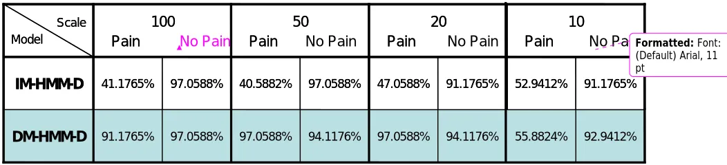
Table 5.1 provides a comparative list of the classification performance results obtained from

the IM-HMM-D and DM-HMM-D schemes. When performance is calculated as an average value

using both classes, the IM-HMM-D system delivers 69.11765% with M=20; and a maximum

72.0588% with M=10. The relatively low performance of IM-HMM-D in classifying pain can be

explained in terms of the substantial inter-dependencies which exist between certain channels and

which this system fails to take into consideration. Considerably higher classification accuracy rates

are obtained by applying the DM-HMM-D system, see Table 5.1. This improved performance is

obtained for all values of M and the system operates best (with a performance in excess of 95%) with

M values in the region of 20 to 50. Note that when several different models provide similar

classification performance, structure with lower values of M and N are preferred due to lower system

complexity. Thus the model with M=20 and N=10 is used below to obtain the “usage rate” for each

EEG channel and hence an indication of the significance of each channel.

Note that, some sequences can be completely blocked out, if necessary, from the resulting

likelihood probability P by setting a minimum threshold Wthreshold that operates during classification on

Wthreshold =10-5_{. Figure 5.2 shows the usage rate of each input channel (feature) as calculated from a}

classification experiment with DM-HMM-D. In this figure certain channels (for example, Channels 4,

6, 15, 16, 39, 48, 49, 51, and 58) are heavily involved in the classification of both Pain and No Pain

conditions. In general, this input channel categorization methodology can be particularly useful to

researchers interested in the reduction of the number of input channels (features) presented at the

input of a classifier with a carefully controlled effect on classification performance.

Experimentation with the novel eClass system involved a data-set of 355 Pain and 355 No-Pain

epochs, in order to produce the fuzzy rule-base of the classifier. As before, these epochs came from

the first 8 out of the available 9 EEG data-sets (experiments). Thus 710 signal epochs were introduced

to the system together with their respective Pain/No Pain labels, (ground-truth). It should be noted that

the eClass approach does not need to be pre-trained, but in order to compare the performance of the

two methods; the same experimental conditions were used here. In this way the system produced a

“rule-set” for each of the Pain and No-Pain conditions, by comparing spatial proximities between

signals of the same class. Following the merging of these two individual “rule-sets”, the system was

ready to classify unknown signals based on the “global rule-set” that contained a total of 168

prototypical EEG signals (rules).

In order to test the classification efficiency of the resulting system, 34 epochs from each class

taken from the 9th _{data-set that was used for testing the system, were presented to eClass.}

Classification was thus performed by comparing the distances formed between the input test EEG

signals and the prototypes stored in the “rule-set”.

Two different approaches were then used in order to arrive at the required classification decision:

1. A “winner takes all” classification approach (see equation 4.2a).

2. A weighted average approach (see equation 4.2b).

Using the first approach, eClass yielded a respectable 79.45% average classification accuracy rate.

experimental results illustrated that employing the “aggressive” winner-takes-all type of decision

outperforms the version that is based on the weighted type of classification. It should be noted that a

classification accuracy of 88.24% is achieved for the No-Pain class whereas the corresponding result

for the Pain condition is 69.21%. This can be associated to the observation that the number of rules

formed by the system when modelling No-Pain EEG signals is significantly larger than that of the

Pain case. Note that the eClass approach does not require the number of prototypes to be

pre-specified; instead prototypes are formed according to the characteristics of the input signals and as a

result of an evolving design procedure. The reason why more clusters and hence prototypes are

obtained in the No-Pain case can be traced to the higher variance of the EEG signals recorded under

the Pain condition, as compared to those recorded under No-Pain. Higher variance (Figure 4.1b) leads

to lower potentials (equation (4.4)) which in turn restricts the process of generating new prototypes.

6. CONCLUSIONS

Two novel and substantially different approaches to the problem of automatically deciding on the

Pain/No Pain condition of a subject using EEG signals are introduced in the paper. The first approach,

DM-HMM-D, is based on a new formulation of a bank of HMM with discrete density classifiers

where each HMM operates on a different channel. Furthermore DM-HMM-D exploits any

inter-dependencies that may exist between the EEG signals of different channels via the introduction per

HHM model of a varying with time weighting function that represents the instantaneous importance

of each channel. This system performs substantially better than the conventional IM-HMM-D

approach and with a Pain/No Pain classification accuracy of 94% and 97% respectively. Whereas this

HMM based approach to EEG Pain/No Pain condition classification requires off-line supervised

training of the system, in order to specify the model parameters whose architecture is fixed (and

should be therefore determined via experimentation), the second classification approach, i.e. eClass, is

far more flexible and defines its fuzzy rule-based structure on line and in response to the input EEG

major asset of eClass and an important differentiator, with respect to other off-line, fixed structure

classification systems, since it opens up significantly the way that the classifier can be used in

practical real-time applications. Furthermore experimental results clearly demonstrated the potential

of the eClass system whose underlining methodology bears the promise of further significant research

developments on supervised on line classification systems.

7. ACKNOWLEDGEMENTS

The authors acknowledge the use of the EEG data courtesy of Hope Hospital, Manchester. The second

author acknowledges the partial support by the Lancaster University of grant ‘EvoMAP’ SBA 7662

REFERENCES

[1] J.R. Wolpaw, D.J McFarland, Multichannel EEG-based brain-computer communication,

Electroencephalography and Clinical Neurophysiology 90, 444-449 (1994).

[2] S.W.G. Derbyshire, Jones A.K.P., “Cerebral responses to a continual tonic pain stimulus

measured using positron emmision tomography”, Pain 76 (1998) 127 – 135.

[3] P. Rappelsberger, Petsche H: “Probability Mapping: Power and Coherence Analyses of

Cognitive Processes”, Brain Topography, 1988, 1: 46-54.

[4] Chen A.-C.N., Rappelsberger P: “Brain and Human Pain: Topographic and Coherence

Mapping”, Brain Topography, 1994, 7, No 2: 129-140.

[5] L.K.Stergioulas, Reoullas M., Xydeas C.S., Baltas E., Bentley D., Youell P., Jones A.:

“Coherence Pattern Classification Using LVQs For Pain Detection”, Analysis of Biomedical

Signals and Images, 16th Biennial International EURASIP Conference BIOSIGNAL 2002

[6] D.E. Bentley., P.D. Youell., A.K.P. Jones.: “Anatomical localization and intra-subject

reproducibility of laser evoked potential source in cingulated cortex, using a realistic head

model”, Clinical Neurophysiology 113 (2002) 1351 – 1356.

[7] J. Bilmes, A Gentle Tutorial of the EM Algorithm and its Application to Parameter Estimation

for Gaussian Mixture and Hidden Markov Models, Tech. Report, International Computer

Science Institute, Berkeley, 1997.

[8] L. R. Rabiner, A Tutorial on Hidden Markov Models and Selected Applications in Speech

Recognition, Proc. of the IEEE,77 (2), 257-286 (1989).

[9] Z. Ghahramani, An Introduction to Hidden Markov Models and Bayesian Networks,

International Journal of Pattern Recognition and AI, 15 (1), 9-42 (2001).

[10]Y. Bengio, Markovian Models for Sequential Data, Neural Computer Surveys, Dept. of

Information and Research Operation, 2, 129-162 (1999).

[11]M. A. Mohamed, P. Gader, Generalized Hidden Markov Models-Part I: Theoretical

Frameworks, IEEE Transaction on Fuzzy Systems, 8 (1), (February 2000).

[12]M. A. Mohamed, P. Gader, Generalized Hidden Markov Models-Part II: Application to

Handwritten Word Recognition, IEEE Transaction of Fuzzy Systems, 8 (1), (February 2000).

[13]K. F. Lee, Automatic Speech Recognition: the development of the SPHINX system, Kluwer

Academic Publish, (1989).

[14]P. Angelov, D. Filev, An approach to on-line identification of evolving Takagi-Sugeno

models, IEEE Trans. on Systems, Man and Cybernetics, part B, 34 (1), 484-498 (2004).

[15]N. Kasabov, Q. Song, DENFIS: Dynamic Evolving Neural-Fuzzy Inference System and Its

[16]S.-Y. Chiao, C. S. Xydeas, Using Hierarchical HMMs in Dynamic Behaviour Modelling,

Proceedings of Seventh International Conference on Information Fusion, Fusion 2004,

Stockholm Sweden, 576-582 (2004).

[17]S.-Y. Chiao, C. S. Xydeas, Behaviour Modelling Using a Hierarchical HMM Approach, IEEE

Computer Society Press Proceedings, (May 2005 to appear).

[18]R. R. Yager, D. P. Filev, Essentials of Fuzzy Modeling and Control, NY: John Wiley (1994).

[19]P.P. Angelov, Evolving Rule-based Models: A Tool for Design of Flexible Adaptive Systems,

Springer, Physica-Verlag, Heidelberg, Germany (2002).

[20]R. O. Duda, D. G. Stork, P. E. Hart, Pattern Classification and Scene Analysis: Pattern

Classification, 2nd _{edition, John Wiley, NY (2001).}

[21]J. Bezdek, Cluster Validity with Fuzzy Sets, Journal of Cybernetics, 3(3), 58-71 (1974).

[22]I. Gath, A.B. Geva, Unsupervised optimal fuzzy clustering, IEEE Trans, Pattern Analysis and

Machine Intelligence, 7, 773-781 (1989).

[23]S.L. Chiu, Fuzzy Model Identification based on Cluster Estimation, Journal of Intelligent and

Fuzzy Systems, 2, 267-278 (1994).

[24]N. Kasabov, Evolving fuzzy neural networks for on-line supervised/unsupervised

knowledge-based learning, IEEE Trans. SMC - part B, Cybernetics31, 902-918 (2001).

[25]D. Carline , P. Angelov, R. Clifford, Agile Collaborative agents for classification of

under-water targets, Undersea Defence Technology, 21-23 June 2005, Amsterdam, The Netherlands.

[26]P. Angelov, An Approach for Fuzzy Rule-base Adaptation using On-line Clustering,

International Journal of Approximate Reasoning, Vol. 35 (3), March 2004, Pages 275-289.

[27]L. Kuncheva, How Good are Fuzzy If-Then Classifiers, IEEE Transactions on Systems, Man

[image:24.612.203.364.101.295.2]

Figure 2.1: EEG cap in its physical form mounted on the scalp of a subject

[image:24.612.171.392.395.590.2]

[image:25.612.154.384.80.196.2]

Figure 3.1: A general HMM structure with

N

hidden states and

M

possible observations per

state.

S₁ S₂ S₃

…

S_N

O₁

O₂

O_M

:

O₁

O₂

O_M

:

O₁

O₂

O_M

:

O₁

O₂

O_M

:

…

States

oT(1) … o2(1)

o1(1) o2(1) … oT(1) o1(1)

o_T(2) … o₂(2)

o₁(2) _o

T(2) … o₂(2) o₁(2)

oT(C) … q2(C)

o1(C) q2(C) … oT(C) o1(C)

HMM#1

HMM#2

HMM#C

P(O(2)_|λ 2) (a)

…

P(O(C)_|λ C)

P(O(1)_|λ 1)

o_T(1) … o₂(1)

o₁(1) _o

T(1) … o₂(1) o₁(1)

o_T(2) … o₂(2)

o₁(2) _o

T(2) … o₂(2) o₁(2)

o_T(C) … q₂(C)

o₁(C) _o

T(C) … q₂(C) o₁(C)

HMM#1

HMM#2

HMM#C

(b)

…

P(O(1)_{| )}

1 ˆ

λ

P(O(2)_{| )}

P(O(C)_{| )}

2 ˆ

λ

C

λ

ˆ

o_T(1) … o₂(1)

o₁(1) _o

T(1) … o₂(1) o₁(1)

o_T(2) … o₂(2)

o₁(2) _o

T(2) … o₂(2) o₁(2)

o_T(C) … q₂(C)

o₁(C) _o

T(C) … q₂(C) o₁(C)

HMM#1

HMM#2

HMM#C

(c)

P(O(1)_|O)

P(O(2)_|O)

P(O(C)_|O)

…

P(O(1)_{| )}

1 ˆ

λ

P(O(2)_{| )}

P(O(C)_{| )}

2 ˆ

λ

C

λ

ˆ

o_T(1) … o₂(1)

o₁(1) _o

T(1) … o₂(1) o₁(1)

o_T(2) … o₂(2)

o₁(2) _o

T(2) … o₂(2) o₁(2)

o_T(C) … q₂(C)

o₁(C) _o

T(C) … q₂(C) o₁(C)

DM-HMM-D-2#1

(d)

DM-HMM-D-2#2

DM-HMM-D-2#C

…

P(O(1)_{| )}

1 ˆ

λ

P(O(2)_{| )}

P(O(C)_{| )}

2 ˆ

λ

[image:26.612.72.377.84.623.2]

C

λ

ˆ

Figure 3.2: (a) a conventional IM-HMM-D, (b) (c) and (d) DM-HMM-D equivalent

0 50 100 150 200 250 300 350 400 450 500 -10

-8 -6 -4 -2 0 2 4 6 8 10

Prototype of Class NoPain

Sampling Instances of the EEG signals

Am

pl

it

ude i

n

m

icr

ov

ol

ts

EEG

1 1

EEG

2 1

Sample l

EEG

3 1

EEG

4 1

Figure 4.1 (a) Prototype EEG signals for the class No Pain for one of the channels

0 50 100 150 200 250 300 350 400 450 500

-15 -10 -5 0 5 10 15

Prototype of Class Pain

Sampling Instances of the EEG signals

A

m

pl

it

u

de i

n

m

icr

ovol

ts

EEG

1 1

EEG

4 1

EEG

3 1

EEG

2 1

[image:27.612.110.481.91.328.2]

Figure 4.1 (b) Prototype EEG signals for the class Pain for the same channel

Figure 4.2

A snap-shot of the clustering for certain moment of time

l

after discretization

[image:28.612.101.462.114.323.2]

of EEG signals for the two channels

Figure 4.3: General Model of the eClass scheme.

EEG1

EEG2

*

*

*

* *

*

Legend:

Class ‘Pain’

Class ‘No-Pain’

.

value of the EEG signal for time instant l

* value of the prototype for time instant l

.

.

.

.

.

.

. .

.

. ..

.

.

.

. .

.

.

.

Class1 Classm

EEG signal selected as a prototype for Class1

EEG signal selected as a prototype for Classm

Classification result ...

Overall Rule-base

1 1

R

1 1 R

R

m

R₁

m

Rm

R

EEG

vector

[image:28.612.116.451.403.563.2]

[image:29.612.123.436.125.300.2]

Figure 5.1: Design and evaluation procedures in EEG classification experiments using

HMMs

Table 5.1: Classification results for the IM-HMM-D and DM-HMM-D systems.

Classification performance is expressed as the percentage of correctly classified EEG

segments

Training Data Set

Scale Quantization

(M=100,50,20,10)

Training IM-HMM-D

Training DM-HMM-D

IM-HMM-D Parameter sets

DM-HMM-D Parameter sets

Testing Data Set

Scale Quantization

(M=100,50,20,10)

IM-HMM-D Recognition Results

IM-HMM-D Parameter sets

DM-HMM-D Parameter sets

DM-HMM-D

Recognition Results Selected Channels _Information

91.1765% 52.9412%

91.1765% 47.0588%

97.0588% 40.5882%

97.0588% 41.1765%

IM - HMM - D

94.1176% 97.0588%

50

Pain No Pain

97.0588% 91.1765%

100

Pain No Pain

92.9412% 55.8824%

94.1176% 97.0588%

DM - HMM - D

10

Pain No Pain 20

Pain Scale

Model

91.1765% 52.9412%

91.1765% 47.0588%

97.0588% 40.5882%

97.0588% 41.1765%

IM - HMM - D

94.1176% 97.0588%

50 Pain

97.0588% 91.1765%

100 Pain

92.9412% 55.8824%

94.1176% 97.0588%

DM - HMM - D

10 Pain 20

Pain No Pain Scale

Model _{Formatted: Font:}

[image:29.612.69.595.387.507.2]

0 10 20 30 40 50 60 0

20 40 60 80 100

Index of Channel

Us

a

g

e

R

a

te

(

%

)

0 10 20 30 40 50 60 0

20 40 60 80 100

Index of Channel

Us

a

g

e

R

a

te

(

%

)

Pain Signal

[image:30.612.89.430.95.368.2]

No-Pain Signal