Cardiac Biometric Identification using Phonocardiogram
Signals by Binary Decision Tree based SVM
K. Lakshmi Devi
Mother Teresa Women’s University, Kodaikanal, Tamil Nadu, India.
M. Arthanari,
Ph.D.Department of Science & Humanities, Nehru Institute of Technology, Coimbatore, Tamil Nadu, India.
ABSTRACT
Analyzing Phonocardiogram signals for Automatic Identification system by Binary Decision Tree based Support Vector Machine is a new approach in the research and this paper examines the applicability of the biometric properties of the Heart Sounds. It is a highly reliable method as it cannot be forged and difficult to disguise. This reduces falsification with highly accurate results. Multi-pass Moving Average Filters (MAF) smoothes the up-sampled DWT coefficients and the peaks are detected by Averaging the Neighbors. Spectral Features are extracted and clustered by HSOM. Rough sets Theory (RST) select the best features for classification. Binary Decision Tree based Support Vector Machine is used as a classifier for recognition and Identification.
Keywords
Phonocardiogram, DWT, Threshold, Self-Organizing Maps, Rough sets, SVM.
1. INTRODUCTION
Reliable authentication and identification is becoming mandatory in recent years in applications such as defense, finance, personnel security and other important fields, where information security is facing issues on illegal copying and sharing of digital media. A biometric system aims at implementing security systems that recognizes a person immediately and certainly. Knowledge-based or possession based access control methods proved to be immortal. It is difficult to forge biometric traits and they seem to be more powerful. They constitute a strong and reasonably permanent link between a person and his identity [1].
Cardiac auscultation uses natural signals called Heart sounds for health monitoring and diagnosis for thousands of years. Heart sounds contain great information to provide unique identity for each person. The Heart produces two biological signals, the Electrocardiogram (ECG) and Phonocardiogram (PCG). Like ECG readings, these signals are difficult to disguise and therefore reduces falsification.
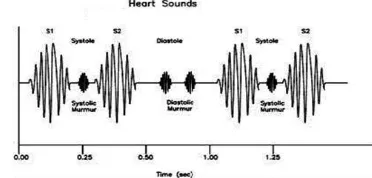
[image:1.595.330.516.256.345.2]Heart sounds are discrete bursts of auditory vibrations of varying Intensity (loudness), frequency (pitch), quality and duration [2]. Two sounds namely S1 and S2 are normally generated as blood flows through the heart valves during each cardiac cycle as shown in Fig 1.
Fig. 1: Time-Frequency representation of Heart Sounds
The first heart sound S1 is low and associated with the vibrations set up by the sudden closure of the mitral tricuspid valve during the ventricles contract and pump blood with the aorta and pulmonary artery at the start of the ventricular systole[3,4]. The second sound S2 is a shorter high-pitched sound caused when the ventricles stop ejecting, relax and allow the aortic and pulmonary valves close just after the end of the ventricular systole. S1 has duration of about 0.15s and the frequency ranges from 25-45Hz. S2 has duration of about 0.12s and ranges from 50-200Hz frequency. The signal has to be manipulated so as to gain useful features that have to involve for the process of identification.
2.
LITERATURE REVIEW
There has been a gradual decline in PCG research, which may be due to the popularity of ECG. However, all these do not confirm all valvular diseases. PCG is an excellent tool for auscultation training and helps in understanding the hemodynamic of the heart [5]. In recent years, different research teams have been studying the possibility of using heart sounds for biometric recognition.
Phua et.al proposed a Novel method based on cepstral analysis of heart sounds for feature extraction, combined with the Gaussian Mixture modeling technique. Francisco Beritelli made a frequency analysis by z-chirp transform (CZT) algorithm. Euclidean distance was used to measure the signal spectra. Later he proposed a multi-band analysis approach to enhance the seperability between intrapersonal and interpersonal classes of values.
Tran et.al worked on the different feature extraction methods, exploring 7 set of features. All features were fed to a feature selection method called RFE-SVM to find the best set of features. Out of which, Gaussian models gave good results.
Fatemian et. al investigated both ECG and PCG for biometric recognition. The heart sounds were processed using Daubecchies 5 wavelets and used two energy (low & high) thresholds to select the coefficients for further stages. The frames were processed by STFT, Mel-frequency filter banks and LDA for dimensionality reduction.
Sumeth et.al segmented cardiac cycles by envelope detection and calculated the length of the signals using auto-correlation of envelope signal. He classified by neural network bagging predictors.
Gill et.al presented a model which detected and identified using Homomorphic envelogram and HMM for feature vectors.
Jasper and Othman computed various energy parameters like Shannon entropy, Shannon energy of different sub-bands taken through DWT. Olmez et.al segmented PCG signals using multi-band wavelet energy (WTE). It gave better performance in comparison with Shannon energy and Homomorphic filtering methods.
3.
METHOD
3.1 Segmentation of S1 and S2
The overall authentication needs manipulation of the signal which involves signal capturing, amplification of the signal and remove noise, changing a signal to emphasize certain characteristics, training and Matching and Identity verification. The raw signal is decomposed into frames of length N ending at time m. Rectangular windowing function chooses frames such that each has one full cardiac cycle of 20ms of frame length and 5ms of overlapping time.
The windowed samples are normalized to remove offsets. Discrete Wavelet Transform (DWT) analyzes the signal at different frequencies with different resolutions. In the process of designing highly personalized gallery templates, a crucial step is the detection of heart beats which are indeed employable for this task. This is because a template signal has to be sufficiently descriptive of the intra-class variability in order for the system to perform robust matching. This issue can be addressed with careful preprocessing of the signal. The discrete wavelet transform (DWT) is chosen for this task, because it provides a dual functionality i.e., it allows for noise reduction and also heart beat delineation using the maxima lines information obtained from the DWT coefficients.
According to Nyquist‟s rule, the signal can be sub-sampled by two, simply by discarding every other sample. The signal is decomposed by Daubechies 5th order wavelet. S1 and S2 fall within the range of frequencies of 30-250Hz. The detailed coefficients of the 3rd, 4th & 5th level (D3, D4 & D5) are taken for the amplification of the signal. The outputs are up-sampled and summed for emphasizing the difference between S1 and S2 sounds.
3.1.1
Multi-pass Moving Average filters
The Heart sound signal still has very complicated patterns with numerous spikes that has little impact on diagnosis but may influence the location of S1 and S2 [6]. Hence the signal is smoothed. If both signal and noise are present, these two can be partially separated by looking at the amplitude of each frequency. The original signal is divided into overlapping
segments as overlap-add method cannot be implemented for filtering signals.
After processing, a smooth window is applied to each of the overlapping segments before they are recombined. This provides a smooth transition of the frequency spectrum from one segment to the next. Moving Average Filters operate by taking the average of the number of points from the Input signal to produce each point in the output signal, given by the equation
𝑦 𝑖 =𝑀1∑ ∑𝑀−1𝑥[𝑖 + 𝑗]
𝑗 =0
Where M is the number of points in the average. The highest amplitude can be attributed and the noise can be discarded, it is set to zero. Multi-pass involves passing the input signal through a MAF two or more times. Two passes are equivalent to using a „triangular‟ smoothing. This is explicitly good smoothing filters. The biggest difference in this filter when compared to others is execution speed. It is the fastest digital filter available. Fig.2 shows the mean, median, max values of the smoothed signal by MAF.
Fig.2: Smoothed signal by MAF showing the mean, median and max values
3.1.2
Peak Detection by Averaging Neighbors
The Peak is the highest point between „valleys‟. It means that there are lower points around it. Slopes greater than zero amplitude are taken into consideration. Let X=[x1, x2, … xi,…xN] be a given uniformly sampled signal containing periodic
peaks, where N is the length of the signal. Let Y= [ y1, y2, …
yi,… yN] be their corresponding amplitudes. xi be the given ith
point in X. The search exists till the length of the signal, from left to right. Let L be the set of k samples of highest amplitude, to the left of the ith point in xi in X. Let R be the set of highest
amplitude to the right of the ith point of xi in X. The peak
function is defined as the average of the maximum of L and R.
F =max L +max R 2
A given point xi in X is a peak if a function
F i, xi ≥ h
Where h is a threshold value obtained by Ma, ven, Genderen and Beukelman(2005) [7]. They compute the threshold automatically as
= (max + 𝑎𝑏𝑠_𝑎𝑣𝑔) 2 + 𝑘 × 𝑎𝑏𝑠𝑑𝑒𝑣
if no. of peaks>1
{
Store peak_dist= current peak position-previous peak Position;
}
Fig.3: Detected S1 and S2 peaks
If the peak distance between the 1st and 2nd peak is greater than the time interval between 2nd and 3rd, then the peaks are named as S2-S1-S1 else it is S1-S2-S1, as the distance between a systole and a diastole is shorter than the distance between a diastole and a systole as in Fig.3.
3.2
Feature Extraction and Selection
The segmented signals are transformed to emphasize certain characteristics. Feature extraction involves simplifying the amount of resources required to describe a large set of data accurately. When performing analysis of complex data, one of the major problems stems from the variables involved. The feature set is reduced in dimensions and called the feature vectors, extracts the relevant information for performing the task. Often it requires a large amount of memory and computation power or a classification algorithm which over fits the training sample.
3.2.1 Extraction
Feature extraction may be temporal or spectral analysis technique. Spectral analysis utilizes spectral representation of the signal for analysis. Grounded on the work in [8] and [9], the following features capture the spectral structures of the signal: Spectral Rolloff, Spectral centroid, Spectral flux and Spectral entropy.
3.2.1.1
Spectral Rolloff
The spectral rolloff measures the spectral shape where the frequency Rt below which 85% of the magnitude distribution is
concentrated
𝑀𝑡[𝑛] 𝑅𝑡
𝑛=1
= 0.85 × 𝑀𝑡[𝑛] 𝑁
𝑛=1
3.2.1.2
Spectral Centroid
The spectral centroid is defined as the center of gravity of the spectrum
𝐶𝑡=
∑𝑁𝑛=1𝑛 ∙ 𝑀𝑡[𝑛] 2
∑𝑁𝑛=1 𝑀𝑡[𝑛] 2
where 𝑀𝑡 𝑛 is the magnitude of the spectrum at frame t and frequency bin n. If the centroid is higher the textures become more brighter.
3.2.1.3
Spectral Flux
The spectral flux is defined as the squared difference between the normalized magnitudes of successive spectral distributions that correspond to successive signal frames
𝐹𝑡= ∑𝑁𝑛=1 𝑁𝑡 𝑛 − 𝑁𝑡−1 𝑛 2
Where Nt[n] and Nt-1[n] are the normalized magnitude of the
Fourier transform at the current time frame t, and the previous time frame t-1, respectively. The spectral flux is a measure of the amount of local spectral change.
3.2.1.4
Spectral Entropy
The spectral entropy measures the energy level as
𝐻 𝑥 = − 𝑝 𝑥𝑖 log2𝑝 𝑥𝑖 𝑁
𝑖=1
If the sequence x[n] is flat, then the output entropy is maximal. Reversely, if the curve displays only one very sharp peak, then the entropy is minimal.
One of the most challenging aspects in clustering is the high dimensionality of most problems. The Spectral Feature coefficients (SFC) are readily used in the voice identification field. The SFC provides a scaling of the frequency spectrum similar to the human ear‟s response. The s1-sound and S2-sound Spectral Coefficients, extracted with a Spectral Features method, is used to characterize the sound.
Fig.4: Feature extraction using DCT and DWT
The dimensionality of the data is reduced by the use of the discrete cosine transform (DCT) and the features extracted by DCT and DWT are differentiated in Fig.4. It extracts the Spectral Features for each sound and removes the remaining noise Channels.
The k-means clustering is executed on the Spectral features to extract two groups (s1 and s2 group) of -the heart sound components.
The clustering data is first partitioned into three groups:
(1) a finite set of objects (Signal Length)
(2) the set of attributes (s1 and s2 features, variables)
(3) the domain of attribute. (Positive or negative)
As Self-Organizing Map (SOM) has the capability of detecting small differences between objects, it has proved to be a useful and efficient tool in finding multivariate data outliers [10-12]. A self-organizing map consists of components called nodes or neurons. Associated with each node is a weight vector of the same dimension as the input data vectors and a position in the map space. The usual arrangement of nodes is a two-dimensional regular spacing in a hexagonal or rectangular grid. The self-organizing map describes a mapping from a higher-dimensional input space to a lower-higher-dimensional map space.
Fig.5: Spatial Clustering using SOM
The procedure for placing a vector from data space onto the map is to find the node with the closest (smallest distance metric) weight vector to the data space vector.
A hierarchical self-organizing map (HSOM) is a type of artificial neural network (ANN). It is an unsupervised learning method to produce a low-dimensional discretized representation of the input space of the training samples, called a map. Hierarchical self-organizing maps are different from other artificial neural networks in the sense that they use a neighborhood function to preserve the topological properties of the input space. HSOMs operate in two modes: training and mapping. “Training” builds the map using input examples. It is a competitive process, which is also called vector quantization. "Mapping" automatically classifies a new input vector. The key idea of the hierarchical self-organizing map (HSOM) is to use a hierarchical structure of multiple layers where each layer consists of a number of independent self-organizing maps (SOMs). One SOM is used at the first layer of the hierarchy. This principle is repeated with the third and any further layers of the HSOM.
First, the number of map units is determined. It uses a heuristic formula of „munits = 5*dlen^0.54321‟. A bigmap is four times the default number of map units. The „mapsize‟ argument influences the final number of map units. After the number of map units has been determined, the map size is determined. Basically, the two biggest Eigen values of the training data are calculated and the ratio between side lengths of the map grid is set to this ratio.
The SOM is trained in two phases: first rough set training and then fine-tuning. The average quantization error and topographic error of the final map are calculated. Finally trained map structure is obtained. A HSOM require less computational effort when compared to a standard SOM and better suited to model a problem that has, by its own nature, some sort of hierarchical structure. Fig.5 depicts the output of clustering through SOM.
3.2.2
Feature Selection
The Rough test feature selection is the process of finding a subset of s1s2 features, from the original set of k-means cluster pattern, optimally according to the defined criterion. Rough sets theory is based on the concept of an upper and a lower approximation of a set, the approximation space and models of sets as shown in Fig.6.
Fig.6 Lower and Upper Approximations of a Set
An information system can be represented as,
𝑠 = 𝑈, 𝐴, 𝑉, 𝑓
where U is the universe, a finite set of N objects (x1, x2, …, xN)
(a nonempty set), A is a finite set of attributes, V = UaAVa
(where Va is a domain of the attribute a), f : U × A → V is the
total decision function (called the information function) such that f(x, a) Va for every a A, x U. B subset of attributes B
Q defines an equivalence relation (called an indiscernibility (unnoticeable) relation) on U
𝐼𝑁𝐷 𝐴 = 𝑥, 𝑦 ∈ 𝑈; ∀𝑎 ∈ 𝐵; 𝑓 𝑥, 𝑎 = 𝑓 𝑦, 𝑎 ,
denoted also by A’. The information system can also be defined as a decision table
𝐷𝑇 = 𝑈, 𝐶 ∪ 𝐷, 𝑉, 𝑓
where C is a set of condition attributes, D is a set of decision attributes, V = UaCDVa, where Va is the set of the domain of
an attribute a Q, f : U × (C D) → V is a total decision function (information function, decision rule in DT) such that f(x, a) Vq for every a A and x V.
The straightforward feature selection procedures are based on an evaluation of the predictive (Entropy) power of individual features, followed by a ranking of such evaluated features and eventually the choice of the first best m features.
A criterion applied to an individual feature could be either of the open-loop or closed-loop type. It can be expected that a single feature alone may have a very low predictive power, whereas when put together with others, it may demonstrate a significant predictive power [13].
3.3 Classification
The SVM-Binary Logical Decision Tree method that is proposed is based on recursively dividing the spectral features in two disjoint groups in every node of the decision tree (true or false) and training a SVM that will decide in which of the groups the incoming unknown sample should be assigned. Fig.7 shows the class and the corresponding decision boundary.
The feature classes from the first k-means clustering group are being assigned to the first (left) sub-tree, while the classes of the second clustering group are being assigned to the (right) second sub-tree. This method uses multiple SVMs arranged in a Logical decision binary tree structure.
3.3.1
Training
A Binary SVM in each node of the tree is trained feature using two of the classes. The verification algorithm then employs probabilistic outputs to measure the similarity between the remaining samples and the two classes used for training.
All training samples in the node are assigned to the two sub-nodes derived from the previously selected classes by similarity. This step repeats at every node until each node contains only samples from one class. The main problem that should be considered seriously here is training time, because aside training, one has to test all samples in every node to find out which classes should be assigned to which sub-node while building the tree. This may decrease the training performance considerably for huge training datasets.
The division of the feature space depends on the structure of a decision tree, and the structure of the tree relate closely to the performance of the classifier [14]. Distance measures such as the Euclidean distance are often used as seperability measures between classes, but the distance between class centers cannot reflect the structure of the classes if the distribution of the classes is not taken into consideration. The novel algorithm of First order logical decision algorithm considers the distribution of classes along with the distances of class centers. These algorithms can help to build a pattern recognition model for classify the signals and increase the efficiency of the training and testing time of data.
3.3.2
Testing
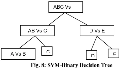
[image:5.595.55.246.484.594.2]The identification (close set) approach, the multi-class Binary-SVM is developed as in Fig.8. Basically, the multi-class binary-SVM can be done by either OAO-binary-SVM (One-Against-One) or OAA (One-Against-All) method.
Fig. 8: SVM-Binary Decision Tree
The feature set is then defined separately for each binary SVM. The number of binary SVMs for OAO-SVM (One-Against-One) and OAA (One-Against-All) are N(N − 1)/2 and N respectively. However, these approaches are very expensive in the evaluation as all the feature extraction methods must be performed. In this work, we developed a multi-class first order Binary decision SVM which is able to select a unique feature set for the whole system. This is done by averaging over the ranking criterion for each component, noted by,
𝐽𝑖 = 𝑤𝑖 𝑘
max
𝑗 𝑤𝑗 𝑘 𝑘
2
where k is the index of the k-th binary Binary-SVM.
For the verification approaches, the typical binary-SVM can be adopted. In this case, the Binary-SVM is trained for each pair of verifying user and background training model. The best feature set is expected to be specifically subject dependent.
The Otsu‟s automatic thresholding method involves iterating through all the possible threshold values and calculating a measure of spread for the feature levels each side of the threshold, i.e. the signals that either falls in verification. The aim is to find the threshold value where the sum of features spreads is at its minimum. In Otsu‟s method it exhaustively search for the threshold that minimizes the intra-class variance (the variance within the class), defined as a weighted sum of variances of the two classes:
σ2
(t) = D1 (t) σ21 (t) + D2 (t) σ22 (t)
Distances Di are the probabilities of the two classes separated
by a threshold t and σ2i variances of these classes. Otsu shows that minimizing the intra-class variance is the same as maximizing inter-class variance:
σ2between (t) = D
1 (t).D2 (t) [μ1 (t) − μ2 (t)] 2
This is expressed in terms of class probabilities Di and class means μi.
The Otsu threshold segmentation method does not depend on modeling the probability density functions, however, it assumes a bimodal distribution of binary-level values (i.e., if the features approximately fits this constraint (conditions), it will do a good job).
4.
EXPERIMENTAL EVALUATION
Heart sounds are recorded with Digital Stethoscope with 16-bit accuracy and a sampling frequency of 2000Hz. A database of 20 PCG sequences comprising of heart sounds of different pathologies from 20 people, both male and female, are taken for the study. Each sound is a .WAV file and is of 70s of length. The proposed algorithm gave higher accuracies of 95% of S1 and 93% of S2 segmentations.
The segmentation accuracies resulted when tested on a subset of Heart sound database. It is the result of the number of sounds segmented without errors to the total number of heart sounds in the database. Multiple passes will be correspondingly slower, but still very quick. In comparison, Gaussian, triangular filters are excruciatingly slow, because they must use convolution. Not only is the moving average filter very good for many applications, it is optimal for a common problem, reducing random white noise.
The HSOM divides the input data space into several subspaces according to different themes. Each of these themes is viewed as a subspace created by a subset of variables from the dataset. Each of these data spaces is used to train a SOM, and its output will be used to train a final merging SOM. This has the advantage of setting an equal weight for each frame. So is well suited for spatial analysis.
Fig.9 Performance measured by FAR
ABC Vs DE
D Vs E AB Vs C
[image:5.595.311.538.660.741.2]The clustered features are trained using SVM-BDT classifier. The trained data is verified with the raw data and recognized for accuracy. Experimental results show that training phase with SVM-BDT is faster. The False Acceptance rate (FAR) is the probability that the system incorrectly authorizes a non-authorized person, due to incorrectly matching the biometric input with a template. The Proposed Method, during recognition, found to be more accurate and had a very low FAR as shown in Fig.9.
5. CONCLUSION
In this paper, PCG signals are used as a biometric trait for human identity verification. It is a very reliable System as it can be easily used but not simulated. The system is tested for identification with various Heart sounds containing arrhythmias like Mitral regurgitation, Mitral stenosis, aortic regurgitation and stenosis. It showed good results. Further research can be contributed in the direction of reducing time consumption, parallel to the accuracy. Authentication inspite of arrhythmias is more importance. Enhancements can be made to the research considering the changes that may happen years later.
6. REFERENCES
[1] Anil K. Jain, Arun A. Ross, Karthik A. Nandakumar., “Introduction to Biometrics”.
[2] Walker HK, Hall WD, Hurst JW., “Clinical methods: The History, Physical and laboratory Examinations”, 3rd
Edition.
[3] Kokosoon Phua, J. Chen, Tran.H. Louis shue., “Heart Sound as a Biomteric”. In Pattern Recognition Society, 2007.
[4] Mustafa Yamach, Zumray Dokur, Tamer Olmez.,”Segmentation of S1-S2 sounds in Phonocardiogram Records using Wavelet Energies”, IEEE, 2008.
[5] Cota Navin Gupta,Ramasamy Palaniappan, Sundaram Swaminathan, Shankar M. Krishnan., “ Neural Network classification of homomorphic segmented heart sounds”.
[6] Yiqi Deng, peter J.bentley., ”A Robust Heart Sound Segmentation and classification Algorithm using Wavelet Decomposition and Spectrogram”.
[7] Meng Ma, Van Genderen, Peter Beukelman., ”Developing and Implementing peak Detection for real time Image Registration”, 2005.
[8] Lie Lu, Hao Jiang, Hong Jiang Zhang.,” A Robust Audio Classification and Segmentation Method”.
[9] S. rossignol, X. Rodett, J. Soumagne, J. L. Collette, P. Depalle, “ Feature Extraction and temporal segmentation of acoustic signals”.
[10] Munoz.A., Muruzabal .j., “ Self-organizing Maps for outlier detection”, Neuro Computing,1998.
[11] F. Hadzic, T.S. Dillon, H. Tan, “ Outlier detection strategy using the self-organizing map”, Knowledge Discovery and Data Mining: Challenges and Realities, pp. 224-243, 2007.
[12] A. Nag, A. Mitra, S. Mitra, “ Multiple Outlier detection in multivariate data using self-organizing maps”, Computational Statistics, pp. 245-264.
[13] B. Walczk, D. L. Massart, “ Rough Sets Theory”.